N.B.: This blog post has been updated in January 2025 to include the latest developments with the DeepSeek-R1 model.
Reinforcement learning (RL) is an exciting and rapidly developing area of machine learning that significantly impacts the future of technology and our everyday lives. RL is a field separate from supervised and unsupervised learning focusing on solving problems through a sequence or sequences of decisions optimized by maximizing the accrual of rewards received by taking correct decisions.
Table of Contents
Key Concepts in Reinforcement Learning
- Agent & Environment: The learner (agent) interacts with its surroundings (environment)
- Actions & States: Decisions made by the agent and the resulting situations
- Rewards: Feedback signals that guide the learning process
- Policy: The strategy that determines how the agent behaves

Origins in Animal Learning
Key Foundations
- Dual origins in animal learning and optimal control
- Established fundamental principles of trial-and-error learning
- Introduced core concepts of reinforcement in behavior
Key Milestones in Learning and Reinforcement
Law of Effect
Edward Thorndike introduced the Law of Effect, which states:
- Actions leading to satisfaction tend to be repeated.
- Actions causing discomfort tend to be avoided.
- The strength of an effect correlates with the intensity of pleasure or pain.
Reinforcement
Ivan Pavlov formally defined reinforcement as the strengthening of behavioral patterns through time-dependent stimulus relationships.
Operant Conditioning
B.F. Skinner expanded on reinforcement learning with his theory of operant conditioning, introducing the role of rewards and punishments in shaping behavior.
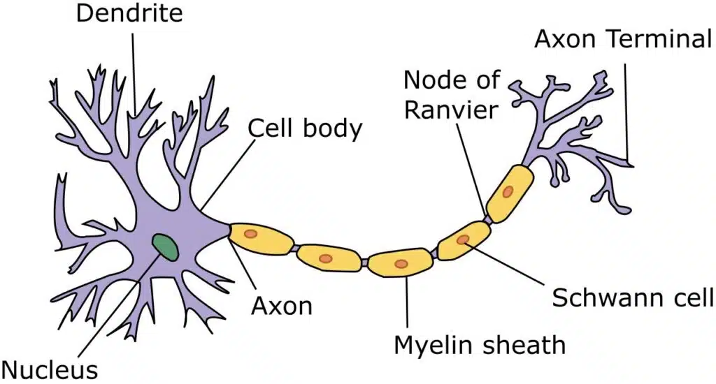
Hebbian Learning
Donald Hebb proposed that “neurons that fire together, wire together,” forming the foundation of modern neural learning and artificial neural networks.
Rescorla-Wagner Model
Robert Rescorla and Allan Wagner developed a mathematical model to describe associative learning, explaining how animals form expectations based on predictive stimuli.
Historical Context
Reinforcement learning originates from two major sources: animal learning and optimal control. Early research in the 20th century focused on understanding how animals adapt behavior through trial-and-error processes.
Edward Thorndike’s experiments with cats in 1911 established the principles of behavioral reinforcement, while Pavlov’s work in 1927 laid the groundwork for stimulus-response associations. Skinner’s operant conditioning (1938) extended these ideas, demonstrating how behavior is shaped through external reinforcements.
By 1949, Donald Hebb introduced the concept of synaptic strengthening, influencing modern neural networks. Finally, the Rescorla-Wagner model (1972) formalized learning dynamics, providing a predictive framework for associative learning.
The Law of Effect, as described by Thorndike, represents one of the most fundamental principles in learning theory. It establishes that an animal will pursue the repetition of actions that reinforce satisfaction and will be deterred from actions that produce discomfort. Furthermore, the greater the level of pleasure or pain experienced, the stronger the resulting behavioral modification.
Impact on Modern RL
The Law of Effect remains central to modern reinforcement learning, influencing:
- Reward function design in RL algorithms
- State-action-reward relationships
- Behavioral policy development
In 1927, Pavlov formalized the term “reinforcement” in the context of animal learning. He described it as the strengthening of a pattern of behavior due to an animal receiving a stimulus – a reinforcer – in a time-dependent relationship with another stimulus or with a response.
Turing’s Unorganised Machines

Key Contributions
- First suggestion of using randomly connected neural networks for computation
- Introduced three types of unorganized machines (A-type, B-type, P-type)
- Proposed machine learning concepts similar to modern neural networks
- Established foundation for trainable computing systems
In 1948, Alan Turing presented a visionary survey of the prospect of constructing machines capable of intelligent behaviour in a report called “Intelligent Machinery”. Turing may have been the first to suggest using randomly connected networks of neuron-like nodes to perform computation and proposed the construction of large, brain-like networks of such neurons capable of being trained as one would teach a child.
Historical Context
Turing’s work on unorganized machines came at a pivotal time when researchers were beginning to explore the possibility of creating machines that could learn. His ideas were remarkably ahead of their time, predating modern neural networks by decades.
While his models were theoretical, they laid the foundation for early computational neuroscience and machine learning. His insights directly influenced later developments such as Minsky’s SNARC (1954), early reinforcement learning models, and even contemporary deep learning architectures.
Key Milestones in Early Machine Learning
Unorganised Machines
Alan Turing proposed the concept of unorganised machines capable of learning through randomness and structured reinforcement.
A-type Machines
Simple networks of randomly connected two-state neurons, forming the basic building blocks of computational models.
B-type Machines
Enhanced versions of A-type machines with organizational mechanisms for improving computational structure.
P-type Machines
Machines designed with “pleasure-pain” responses to mimic human-like learning and behavior shaping.
SNARC
Marvin Minsky developed the first artificial neural network simulator, inspired by biological brain connections.
STELLA System
John Andreae developed a machine that learns through interaction with its environment, an early form of reinforcement learning.
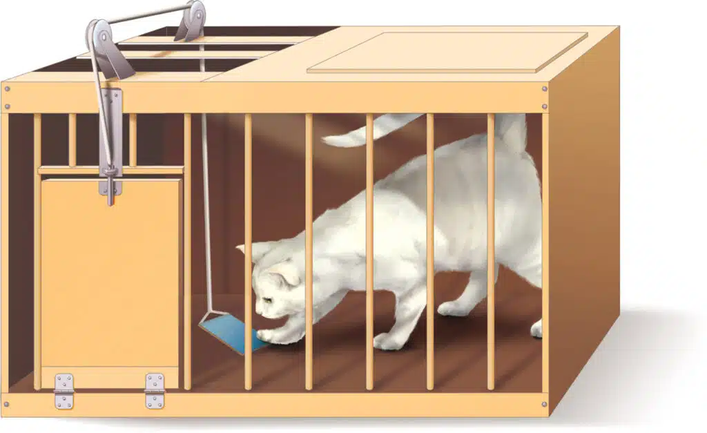
Early Computing Innovations (1933-1954)
Thomas Ross built a machine capable of maze navigation and path memory through switch configurations.
Claude Shannon demonstrated Theseus, a maze-running mouse using magnets and relays for path memory.
Marvin Minsky developed SNARCs (Stochastic Neural-Analog Reinforcement Calculators), inspired by biological neural connections.
Impact on Modern AI
- Influenced the development of artificial neural networks
- Introduced concepts of machine learning through trial and error
- Established the possibility of training machines like human children
- Laid groundwork for reinforcement learning architectures
Trial-and-error learning led to the production of many electro-mechanical machines. Research in computational trial-and-error processes eventually generalized to pattern recognition before being absorbed into supervised learning, where error information is used to update neuron connection weights. Investigation into RL faded throughout the 1960s and 1970s.
However, in 1963, although relatively unknown, John Andreae developed pioneering research, including the STELLA system, which learns through interaction with its environment, and machines with an “internal monologue,” later extending to teacher-guided learning systems.
Origins in Optimal Control
Key Concepts
- Formal framework for optimization in control problems
- Dynamic programming for mathematical optimization
- Introduction of Markovian Decision Processes (MDPs)
- Development of policy iteration methods
Optimal Control research began in the 1950s as a formal framework to define optimization methods to derive control policies in continuous time control problems, as shown by Pontryagin and Neustadt in 1962.
Evolution of Optimal Control Theory
Emergence of optimal control as a formal framework for optimization methods.
Richard Bellman develops dynamic programming and introduces the Bellman equation.
Ronald Howard devises the policy iteration method for Markovian Decision Processes.
Pontryagin and Neustadt formalize control policies in continuous time problems.
Dynamic Programming
Bellman’s method for solving control problems through mathematical optimization and computer programming.
Markovian Decision Process
Discrete stochastic version of the optimal control problem, fundamental to modern RL.
Policy Iteration
Howard’s method for finding optimal policies in MDPs through iterative improvement.
Key Mathematical Elements
- Bellman Equation: Defines optimal value function through dynamic programming.
- Policy Functions: Maps states to actions in control problems.
- Value Functions: Measures the worth of states and actions.
What is the difference between reinforcement learning and optimal control?
Relationship to Reinforcement Learning
The modern understanding appreciates work in optimal control as closely related to reinforcement learning. Key distinctions and overlaps include:
- RL problems are closely associated with optimal control problems, particularly stochastic ones
- Dynamic programming methods are considered reinforcement learning methods
- RL generalizes optimal control ideas to non-traditional problems
- Both share fundamental principles of optimization and decision-making
Optimal Control Focus
- Continuous-time systems
- Precise system models
- Analytical solutions
RL Characteristics
- Discrete and continuous systems
- Model-free learning capability
- Iterative, approximate solutions
Common Ground
- Optimization principles
- Value function concepts
- Policy improvement methods
Learning Automata
Key Concepts
- Adaptive decision-making units in random environments
- Learning through repeated environment interactions
- Probability-based action selection
- Foundation for multi-armed bandit solutions
In the early 1960s, research in learning automata commenced and can be traced back to Michael Lvovitch Tsetlin in the Soviet Union. A learning automaton is an adaptive decision-making unit situated in a random environment that learns the optimal action through repeated interactions with its environment.
Historical Context
Learning automata were developed as a probabilistic alternative to early neural network models. Unlike fixed-rule systems, learning automata continuously adapt their decision-making strategies based on environmental feedback. This approach laid the foundation for solving multi-armed bandit problems, pattern classification, and reinforcement learning models.
As computing power increased, learning automata principles were extended to game theory, genetic algorithms, and deep reinforcement learning, influencing AI applications in robotics, finance, and optimization problems.
Key Developments in Learning Automata
Foundation of Learning Automata
Michael L. Tsetlin develops the fundamental theory of learning automata in the Soviet Union.
Tsetlin Automaton
Introduction of the Tsetlin Automaton, a learning model that adapts through environmental feedback, proving more versatile than artificial neurons.
Early Applications
Learning automata are applied to multi-armed bandit problems, pattern classification, and optimization tasks.
Advancements in Probabilistic Learning
Refinements in stochastic learning models improve convergence rates, leading to applications in control systems and AI decision-making.
Integration into Reinforcement Learning
Learning automata influence multi-agent reinforcement learning (MARL), neuroevolution, and deep reinforcement learning.
Applications of Learning Automata
- Pattern classification systems
- Multi-armed bandit problem solutions
- Decentralized control systems
- Equi-partitioning problems
- Faulty dichotomous search algorithms
Learning automata remain a core element of adaptive AI systems, influencing modern reinforcement learning architectures, robotics, and genetic algorithms. Their ability to iteratively improve decision-making through interaction makes them a cornerstone of intelligent autonomous systems.
Hedonistic Neurons
Key Innovations
- Shift from equilibrium-seeking to maximizing systems
- Individual neurons as pleasure-seeking units
- Local reinforcement in neural networks
- Bridge between neuroscience and machine learning
Development of Hedonistic Neuron Theory
Equilibrium vs. Maximization
Harry Klopf challenges the focus on equilibrium-seeking processes in artificial intelligence, proposing neurons as individual maximizing units.
Hedonistic Neuron Hypothesis
Development of the hedonistic neuron model, suggesting neurons adjust their behavior based on local reinforcement rather than network-wide feedback.
Neuron-Local Law of Effect
Publication of key findings on how individual neurons implement a local version of the law of effect, strengthening rewarded synaptic connections.
Biological Reinforcement Learning
Research in neuroscience uncovers dopamine’s role in reinforcement learning, aligning with the principles of hedonistic neurons.
Influence on AI and RL
Hedonistic neuron principles inspire local learning rules in artificial neural networks, reinforcement learning, and biologically plausible AI architectures.
Distinction from Traditional Approaches
- Equilibrium-Seeking: Traditional supervised learning aims for stable states.
- Maximizing Systems: Hedonistic neurons actively seek to maximize rewards.
- Local vs. Global: Learning occurs at the individual neuron level rather than network-wide.
- Biological Inspiration: Closer alignment with natural neural processes.
Overlap of Neurobiology and Reinforcement Learning
Neurobiological Foundations
Research has identified distinct learning mechanisms within the cortex-cerebellum-basal ganglia system:
- Dopamine’s role in reward prediction error signaling
- Basal ganglia’s function in action selection
- Integration of multiple learning mechanisms
Biological Learning Mechanisms
Dopamine Signaling
Discovery of dopamine’s role in providing reward prediction error signals, influencing learning processes.
Basal Ganglia and RL
Research shows the basal ganglia function as an action selection mechanism guided by dopaminergic feedback, paralleling reinforcement learning algorithms.
Super-Learning Systems
Advancements in AI integrate multiple biological learning mechanisms for adaptive and flexible motor behavior acquisition.
Impact on Modern RL
The hedonistic neuron concept influenced:
- Development of local learning rules in artificial neural networks
- Understanding of biological reinforcement learning
- Design of more biologically plausible AI systems
- Integration of supervised and reinforcement learning approaches
Temporal Difference Learning

Key Concepts
- Prediction-based learning from delayed rewards
- Inspired by mathematical differentiation
- Combines trial-and-error with prediction learning
- Foundation for modern RL algorithms
Temporal Difference (TD) learning is inspired by mathematical differentiation and aims to build accurate reward predictions from delayed rewards. TD predicts the combination of immediate rewards and the future reward estimate at the next time step.
Evolution of Temporal Difference Learning
Klopf’s Early Reinforcement Learning Work
Harry Klopf explores reinforcement learning in large adaptive systems with individual reward-seeking components.
Sutton’s PhD Dissertation
Richard Sutton formally introduces the foundations of Temporal Difference learning.
Introduction of Temporal Difference Learning
Sutton’s definitive paper establishes TD learning as a new paradigm in reinforcement learning.
TD-Gammon Breakthrough
Gerald Tesauro applies TD learning to backgammon, achieving grandmaster-level play using minimal expert knowledge.
Integration with Neural Networks
TD methods are combined with backpropagation, influencing early deep reinforcement learning research.
DeepMind’s AlphaGo
TD learning concepts influence deep reinforcement learning techniques, leading to AlphaGo’s breakthrough in game-playing AI.
TD Learning in AI
Modern AI systems, including robotics, finance, and healthcare, use TD methods for optimizing decision-making in complex environments.
Core TD Learning Process
- Make a prediction about future rewards.
- Observe the actual outcome.
- Calculate the temporal difference error.
- Adjust the old prediction toward the new prediction.
- Repeat the process to improve accuracy.
Key Components of TD Learning
Secondary Reinforcers
TD learning models how secondary reinforcers acquire value through repeated exposure to primary reinforcers.
Actor-Critic Architecture
TD learning is applied in actor-critic models, where one network learns policies and another learns value functions.
Temporal Credit Assignment
TD learning solves the challenge of attributing credit to earlier decisions that led to later successes.
Integration with Neural Networks
Key developments in combining TD methods with neural networks:
- 1983: Applied to pole-balancing problem
- 1984-1986: Integrated with backpropagation
- 1992: TD-Gammon breakthrough
TD-Gammon
Impact of TD-Gammon
Technical Innovation
TD-Gammon combines TD-λ learning with multilayer neural networks, backpropagating TD errors.
Impact on Human Play
TD-Gammon influences human backgammon strategies, showing AI can uncover novel strategic insights.
Legacy in AI Research
TD-Gammon’s success paves the way for later game-playing AI systems such as AlphaGo, AlphaZero, and MuZero.
TD-Gammon Breakthrough
- Developed by Gerry Tesauro in 1992
- Required minimal backgammon knowledge
- Achieved grandmaster-level play
- Combined TD-lambda with neural networks
- Influenced human expert play strategies
Q-Learning
Key Innovations
- Model-free reinforcement learning algorithm
- Direct optimal control learning without transition modeling
- Convergence guarantee for optimal policy
- Foundation for modern deep RL systems
Evolution of Q-Learning
Introduction of Q-Learning
Chris Watkins introduces Q-learning in his PhD thesis “Learning from Delayed Rewards.”
Convergence Proof
Watkins and Dayan publish proof of Q-learning’s convergence under certain conditions.
Deep Learning Revolution
Breakthroughs in deep learning fuel renewed interest in deep Q-learning.
Deep Q-Networks (DQN)
DeepMind introduces deep Q-learning, integrating convolutional neural networks with Q-learning.
Human-Level Atari Performance
DeepMind’s DQN surpasses human performance in several Atari games using a single reinforcement learning algorithm.
AlphaGo’s Impact
AlphaGo, leveraging deep reinforcement learning, defeats world champion Go players.
Deep Q-Learning in Robotics and AI
Q-learning techniques continue advancing in robotics, autonomous systems, and strategic AI applications.
Deep Reinforcement Learning and Deep Q-learning
Neural Network Integration
- Neural networks replace traditional Q-value tables
- Enables handling of complex state spaces
- Allows for better generalization
- Introduces Experience Replay for stable learning
Google DeepMind and Video Games
Breakthrough Achievements
- Mastered multiple Atari games with a single algorithm
- Surpassed human performance in games like Space Invaders and Breakout
- Demonstrated general game-playing capabilities
- Achieved superhuman performance without game-specific knowledge
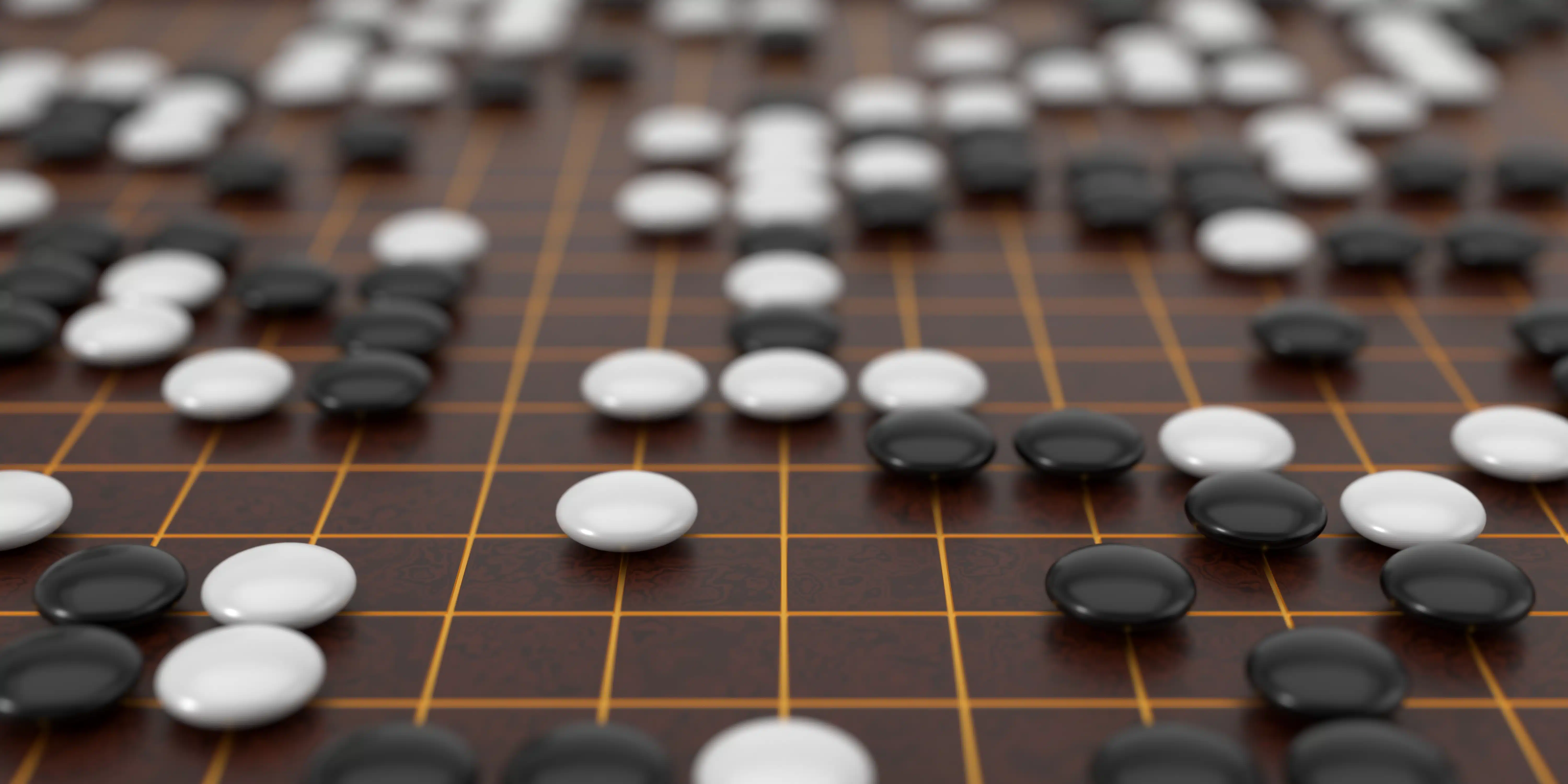
AlphaGo
AlphaGo Milestones
First Victory Against a Professional Player
AlphaGo defeats European Go champion Fan Hui, marking the first AI victory against a pro human player.
Defeats Lee Sedol
AlphaGo defeats 18-time world champion Lee Sedol 4-1 in a historic match.
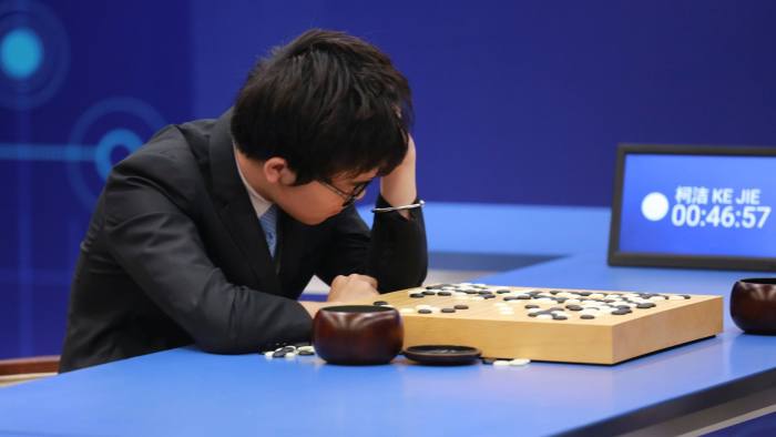
Defeating Ke Jie
AlphaGo defeats world #1 Ke Jie at the Future of Go Summit.
AlphaGo Zero Revolution
AlphaGo Zero, trained exclusively through self-play, defeats the original AlphaGo 100-0 after just three days of training.
AlphaGo Zero Innovation
- Learned solely through self-play
- Required no human game data
- Achieved superhuman performance in days
- Used less computational power than the original AlphaGo
From AlphaGo to AlphaZero
AlphaZero Introduced
DeepMind develops AlphaZero, an AI capable of mastering Go, chess, and shogi using self-play.
Mastering Chess in Four Hours
AlphaZero surpasses Stockfish, the leading chess engine, after only four hours of self-play training.
MuZero Innovation
DeepMind introduces MuZero, capable of mastering complex tasks without an explicit model of the environment.
Impact on AI
- Established reinforcement learning as a dominant paradigm in AI
- Paved the way for AI-driven strategy games and autonomous systems
- Revolutionized self-play and unsupervised training techniques
Modern Developments
Key Breakthroughs
- Application to biomedical research (AlphaFold)
- Advancements in training efficiency
- Pure RL approach with DeepSeek-R1-Zero
- Integration with large language models
The research community is still in the early stages of fully understanding how practical deep reinforcement learning is across multiple domains.
Key Advances in AI and Reinforcement Learning
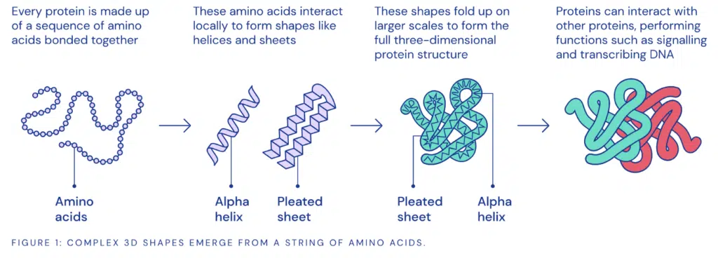
AlphaFold’s Breakthrough
DeepMind’s AlphaFold achieves near-exact protein structure predictions, revolutionizing biomedical research.
Industrial Applications
Reinforcement learning extends to robotics, medical imaging, and autonomous systems.
Training Innovations
Google Brain and DeepMind introduce adaptive reinforcement learning strategies for improving sample efficiency.
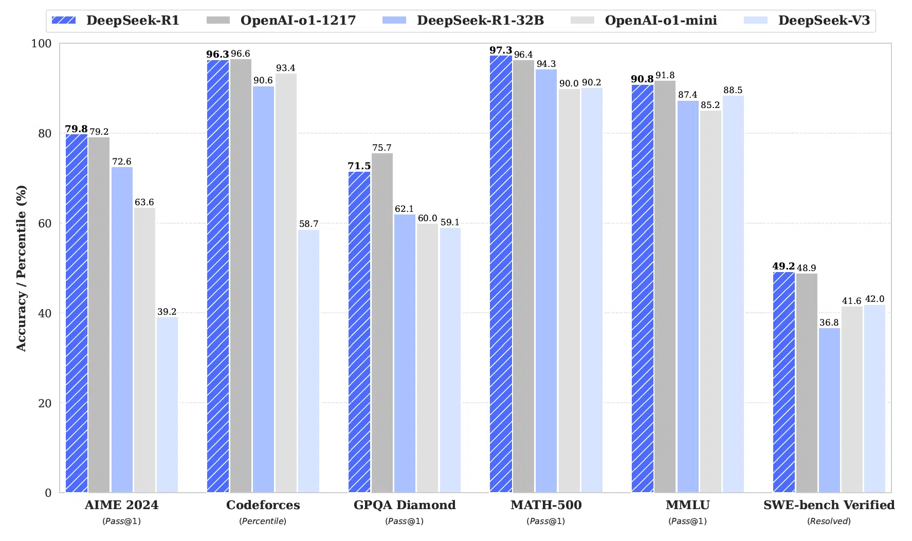
DeepSeek-R1 and Pure RL
DeepSeek-R1-Zero demonstrates that large models can achieve sophisticated reasoning purely through reinforcement learning, reducing training costs dramatically.
RL and Large Language Models
Reinforcement learning increasingly replaces traditional supervised learning for efficient and scalable AI reasoning.
Recent Training Innovations
- Google Brain’s Adaptive Strategy: Optimization through selective information sharing.
- Never Give Up Strategy: DeepMind’s k-nearest neighbors approach for exploration.
- Pure RL Training: DeepSeek-R1-Zero proves reinforcement learning alone can achieve high-level reasoning.
Reinforcement Learning and Large Language Models
Major Research Breakthrough
The integration of reinforcement learning with large language models marks a fundamental shift in AI development. For a comprehensive analysis, see our coverage: DeepSeek-R1: A Breakthrough in AI Reasoning.
AI Training Evolution
Traditional LLM Training
Large language models relied on supervised learning, requiring massive datasets and expensive computation.
DeepSeek-R1 Innovation
Pure reinforcement learning approach achieves state-of-the-art reasoning while dramatically reducing training costs.
AI Democratization
Lower costs enable more researchers and institutions to develop advanced AI models, accelerating innovation.
Key Achievements
- Training Cost Reduction: Decreased from $100M+ to ~$5M while maintaining performance.
- Performance: Achieved state-of-the-art results across multiple reasoning benchmarks.
- Accessibility: Made advanced AI development more feasible for smaller research institutions.
- Efficiency: Demonstrated that pure reinforcement learning can lead to powerful AI models.
Looking Forward
These advancements establish new possibilities for efficient and accessible AI development, potentially accelerating progress across multiple disciplines. For further details, read our comprehensive coverage: DeepSeek-R1: A Breakthrough in AI Reasoning.
Conclusion
Reinforcement learning has an extensive history with a fascinating cross-pollination of ideas, generating research that sent waves through behavioural science, cognitive neuroscience, machine learning, optimal control, and others. This field of study has evolved rapidly since its inception in the 1950s, where the theory and concepts were fleshed out, to the application of theory through neural networks leading to the conquering of electronic video games and the advanced board games Backgammon, Chess, and Go. The fantastic exploits in gaming have given researchers valuable insights into the applicability and limitations of deep reinforcement learning. Deep reinforcement learning can be computationally prohibitive to achieve the most acclaimed performance seen. New approaches are being explored, such as multi-environment training and leveraging language modelling to extract high-level extractions to learn more efficiently.
Whether deep reinforcement learning is a step toward artificial general intelligence (AGI) remains an open question, as RL excels primarily in constrained environments. The biggest challenge lies in achieving generalization. However, AGI does not have to be the ultimate goal of this research. In the coming years, RL will continue to transform various fields, including robotics, medicine, business, and industry. As computing resources become more accessible, innovation in RL will no longer be confined to major tech giants like Google. With a promising trajectory, RL is set to remain a dynamic and influential area of artificial intelligence research.
Thank you for joining us on this journey through reinforcement learning’s history. We hope this article has illuminated both the complexity of RL’s development and its nature as a collaborative field—one that thrives on sharing insights across disciplines, from behavioral science to modern AI, and continues to evolve through this exchange of ideas.
If you found this historical overview valuable, please consider citing or sharing it with fellow researchers and AI enthusiasts. For more in-depth analysis of recent developments, particularly regarding DeepSeek-R1, explore our Further Reading section, including our comprehensive coverage at DeepSeek-R1: A Breakthrough in AI Reasoning.
Further Reading
Foundational Concepts
-
DeepSeek-R1: A Breakthrough in AI Reasoning
Comprehensive analysis of DeepSeek-R1’s development and impact on reinforcement learning in language models, including detailed technical breakdowns and performance evaluations.
-
Law of Effect in Learning Automata
Original work by Thorndike establishing the fundamental principles that would later influence reinforcement learning development.
Historical Development
-
Animal Learning and Neural Networks
Exploration of how biological learning processes influenced the development of artificial neural networks and reinforcement learning systems.
-
Learning from Delayed Rewards (1989)
Watkins’ original PhD thesis introducing Q-learning, a cornerstone of modern reinforcement learning algorithms.
Deep Reinforcement Learning
-
Human-level Control Through Deep Reinforcement Learning
Seminal paper by DeepMind demonstrating the first successful integration of deep learning with reinforcement learning for playing Atari games.
-
Mastering the Game of Go without Human Knowledge
Breakthrough paper describing AlphaGo Zero’s pure reinforcement learning approach to mastering Go.
Modern Applications and Developments
-
AlphaFold: Protein Structure Prediction
Documentation and research papers on AlphaFold’s application of deep learning to protein structure prediction, demonstrating real-world impact of RL techniques.
-
DeepSeekMath: Mathematical Reasoning in Open Language Models
Analysis of mathematical reasoning capabilities in large language models through reinforcement learning approaches.
Implementation Resources
-
Stable Baselines3
Reliable implementations of modern reinforcement learning algorithms with extensive documentation and examples.
-
Keras RL Examples
Collection of reinforcement learning implementations using Keras, including DQN, Actor-Critic, and other modern architectures.
-
OpenAI Gym
Standard toolkit for developing and comparing reinforcement learning algorithms across various environments.
Latest Research Directions
-
Math-Shepherd: Label-free Step-by-Step Verification for LLMs
Research on improving mathematical reasoning capabilities in language models through reinforcement learning techniques.
-
Pushing the Limits of Mathematical Reasoning
Investigation into advanced techniques for mathematical reasoning in open language models using reinforcement learning.
-
DeepSeek-R1: Incentivizing Reasoning Capability in LLMs via Reinforcement Learning
The official research paper detailing DeepSeek-R1’s training methodology, reinforcement learning framework, and performance benchmarks.
-
DeepSeek-V3 Technical Report
A deep dive into DeepSeek-V3, the base model used for DeepSeek-R1, covering its architecture, datasets, and training optimizations.
Attribution and Citation
If you found this guide and tools helpful, feel free to link back to this page or cite it in your work!

Suf is a senior advisor in data science with deep expertise in Natural Language Processing, Complex Networks, and Anomaly Detection. Formerly a postdoctoral research fellow, he applied advanced physics techniques to tackle real-world, data-heavy industry challenges. Before that, he was a particle physicist at the ATLAS Experiment of the Large Hadron Collider. Now, he’s focused on bringing more fun and curiosity to the world of science and research online.