How To Do Bucket Sort in C++

Bucket Sort is a sorting algorithm that distributes elements into a number of “buckets,” sorts the elements within those buckets, and then concatenates the buckets to form the final sorted array. It’s particularly efficient when the input is uniformly distributed over a range. In this blog post, we’ll explore Bucket Sort, understand how it works, and implement it in C++. Additionally, we will compare the performance of Bucket Sort, Counting Sort, and Radix Sort to analyze their strengths and weaknesses.

---

What is Bucket Sort?

Bucket Sort is an efficient sorting algorithm used for sorting real numbers or uniformly distributed integers. The key idea behind Bucket Sort is to partition the input into a number of buckets, where each bucket holds a range of values. The algorithm then sorts each bucket, often using a simpler sorting algorithm like Insertion Sort or Counting Sort, and finally concatenates all the sorted buckets.

Time Complexity:

• Best Case: O(n + k) where k is the number of buckets.
• Average Case: O(n + k) assuming a uniform distribution of elements.
• Worst Case: O(n²) if all elements fall into one bucket.

---

How Bucket Sort Works

The algorithm works as follows:

1. Divide the elements into buckets: Each bucket corresponds to a specific range of values.
2. Sort each bucket: Apply a simple sorting algorithm (often Insertion Sort) to each individual bucket.
3. Concatenate all buckets: Combine the sorted elements from each bucket to get the final sorted array.

Steps:

1. Initialize Buckets: Create an array of empty buckets.
2. Distribute the Elements: Place each element into its appropriate bucket based on its value.
3. Sort the Buckets: Sort each bucket using another sorting algorithm.
4. Concatenate the Buckets: Concatenate all the sorted buckets to form the final sorted array.

---

Bucket Sort Pseudocode

Here’s the pseudocode for Bucket Sort:

BUCKET_SORT(arr, n)
    Input: arr - Array of n elements to be sorted
    Output: Sorted array

    Step 1: Initialize empty buckets
    buckets = array of n empty lists

    Step 2: Put array elements in different buckets
    for i = 0 to n-1 do
        index = bucketIndex(arr[i], n)  // Find the bucket index for arr[i]
        buckets[index].append(arr[i])

    Step 3: Sort individual buckets
    for i = 0 to n-1 do
        sort(buckets[i])  // Sort each bucket using a suitable sorting algorithm (Insertion Sort is common)

    Step 4: Concatenate all buckets into arr[]
    index = 0
    for i = 0 to n-1 do
        for element in buckets[i] do
            arr[index] = element
            index = index + 1

    return arr

Explanation:

• n empty buckets: Buckets are created to store elements based on a range or distribution.
• Insert elements: Each element is placed into the corresponding bucket based on its value.
• Sort buckets: Each bucket is sorted individually using an appropriate sorting algorithm.
• Concatenate: The sorted buckets are combined to produce the final sorted output.

---

Bucket Sort Implementation in C++

Let’s now implement Bucket Sort in C++ with a step-by-step approach.

#include <iostream>
#include <vector>
#include <algorithm> // For sort()
#include <cstdlib>   // For rand()
#include <ctime>     // For seeding random generator

// Function to perform Bucket Sort
void bucketSort(float arr[], int n) {
    // Step 1: Create empty buckets
    std::vector<float> buckets[n];

    // Step 2: Put array elements in different buckets
    for (int i = 0; i < n; i++) {
        // Finding the bucket index (assuming the range of input is [0, 1))
        int bucketIndex = n * arr[i]; // index in the range 0 to n-1
        buckets[bucketIndex].push_back(arr[i]);
    }

    // Step 3: Sort individual buckets
    for (int i = 0; i < n; i++) {
        std::sort(buckets[i].begin(), buckets[i].end());
    }

    // Step 4: Concatenate all buckets into arr[]
    int index = 0;
    for (int i = 0; i < n; i++) {
        for (size_t j = 0; j < buckets[i].size(); j++) {
            arr[index++] = buckets[i][j];
        }
    }
}

int main() {
    // Seed for random number generation
    std::srand(std::time(0));

    // Example of a slightly larger array with 20 floating point numbers in the range [0, 1)
    const int n = 20; // Size of the array
    float arr[n];

    // Populate the array with random float values in the range [0, 1)
    for (int i = 0; i < n; i++) {
        arr[i] = static_cast<float>(rand()) / static_cast<float>(RAND_MAX);
    }

    // Print the original array
    std::cout << "Original array: \n";
    for (int i = 0; i < n; i++) {
        std::cout << arr[i] << " ";
    }
    std::cout << "\n\n";

    // Perform Bucket Sort
    bucketSort(arr, n);

    // Print the sorted array
    std::cout << "Sorted array: \n";
    for (int i = 0; i < n; i++) {
        std::cout << arr[i] << " ";
    }
    std::cout << std::endl;

    return 0;
}

Output:

Original array: 
0.818861 0.59845 0.143636 0.0894762 0.827274 0.989457 0.798861 0.461329 0.56165 0.646899 0.423003 0.415834 0.922704 0.890925 0.783134 0.127218 0.153907 0.721588 0.736764 0.796315 

Sorted array: 
0.0894762 0.127218 0.143636 0.153907 0.415834 0.423003 0.461329 0.56165 0.59845 0.646899 0.721588 0.736764 0.783134 0.796315 0.798861 0.818861 0.827274 0.890925 0.922704 0.989457 

What Algorithm Does std::sort() Implement?

The std::sort() function in C++ uses Introspective Sort (Introsort). Introsort is a hybrid sorting algorithm that combines three different algorithms based on the input data:

1. Quick Sort: Initially, std::sort() uses Quick Sort for most of the sorting process.
2. Heap Sort: If the recursion depth in Quick Sort becomes too large (indicating a potential worst-case scenario), it switches to Heap Sort to ensure a worst-case time complexity of O(n log n).
3. Insertion Sort: When the size of the subarrays is small (typically less than 16 elements), std::sort() switches to Insertion Sort, as it’s more efficient for small datasets.

Step-by-Step Process of Bucket Sort

Let’s go through a step-by-step walk-through of how Bucket Sort works on the original array. For this example, we’ll take an array with 10 elements and sort it using Bucket Sort.

Original Array:

arr[] = {0.42, 0.32, 0.23, 0.52, 0.25, 0.47, 0.51, 0.37, 0.33, 0.29}

1. Initialize Empty Buckets:

• The number of buckets is typically chosen based on the number of elements in the array. In this case, we will create 10 buckets (since the size of the array is 10).
• Each bucket will be represented by an empty list (in practice, a dynamic array like std::vector).

Buckets (Initially empty):

bucket[0] = []
bucket[1] = []
bucket[2] = []
bucket[3] = []
bucket[4] = []
bucket[5] = []
bucket[6] = []
bucket[7] = []
bucket[8] = []
bucket[9] = []

2. Distribute Array Elements into Buckets:

• We distribute the elements of the array into buckets based on their values. Since the values are between 0 and 1, we multiply each value by 10 to determine the bucket index (assuming the range is [0, 1)).
• Formula: bucketIndex = n * arr[i], where n = 10 in this case.

Bucket Assignment:

• For arr[0] = 0.42, the index is 10 * 0.42 = 4, so it goes into bucket[4].
• For arr[1] = 0.32, the index is 10 * 0.32 = 3, so it goes into bucket[3].
• For arr[2] = 0.23, the index is 10 * 0.23 = 2, so it goes into bucket[2].
• For arr[3] = 0.52, the index is 10 * 0.52 = 5, so it goes into bucket[5].
• For arr[4] = 0.25, the index is 10 * 0.25 = 2, so it also goes into bucket[2].
• For arr[5] = 0.47, the index is 10 * 0.47 = 4, so it goes into bucket[4].
• For arr[6] = 0.51, the index is 10 * 0.51 = 5, so it goes into bucket[5].
• For arr[7] = 0.37, the index is 10 * 0.37 = 3, so it goes into bucket[3].
• For arr[8] = 0.33, the index is 10 * 0.33 = 3, so it goes into bucket[3].
• For arr[9] = 0.29, the index is 10 * 0.29 = 2, so it goes into bucket[2].

Buckets After Distribution:

bucket[0] = []
bucket[1] = []
bucket[2] = [0.23, 0.25, 0.29]
bucket[3] = [0.32, 0.37, 0.33]
bucket[4] = [0.42, 0.47]
bucket[5] = [0.52, 0.51]
bucket[6] = []
bucket[7] = []
bucket[8] = []
bucket[9] = []

3. Sort Individual Buckets:

• We now sort each bucket individually. You can use any sorting algorithm (like Insertion Sort or Quick Sort). Here, for simplicity, we’ll assume std::sort() is used, which sorts each bucket in ascending order.

Sorted Buckets:

• bucket[2] (already sorted): [0.23, 0.25, 0.29]
• bucket[3] (sorted): [0.32, 0.33, 0.37]
• bucket[4] (already sorted): [0.42, 0.47]
• bucket[5] (sorted): [0.51, 0.52]

bucket[0] = []
bucket[1] = []
bucket[2] = [0.23, 0.25, 0.29]
bucket[3] = [0.32, 0.33, 0.37]
bucket[4] = [0.42, 0.47]
bucket[5] = [0.51, 0.52]
bucket[6] = []
bucket[7] = []
bucket[8] = []
bucket[9] = []

4. Concatenate Buckets:

• Finally, we concatenate all the elements from the sorted buckets into the original array. The result is a fully sorted array.

Concatenation Process:

• Start by placing the sorted elements from bucket[2] into the array: [0.23, 0.25, 0.29]
• Then, add the elements from bucket[3]: [0.32, 0.33, 0.37]
• Then, add the elements from bucket[4]: [0.42, 0.47]
• Finally, add the elements from bucket[5]: [0.51, 0.52]

Final Sorted Array:

arr[] = {0.23, 0.25, 0.29, 0.32, 0.33, 0.37, 0.42, 0.47, 0.51, 0.52}

Summary of Steps:

1. Create Buckets: Initialize empty buckets based on the size of the array.
2. Distribute Elements: Place each element into its respective bucket based on its value.
3. Sort Buckets: Sort the elements within each bucket individually.
4. Concatenate: Combine all the sorted buckets into the original array to get the final sorted array.

---

Advantages of Using Bucket Sort

1. Efficient for Uniformly Distributed Data
   Bucket Sort is particularly efficient when the input data is uniformly distributed across a known range. By dividing the data into evenly distributed buckets, Bucket Sort can significantly reduce the number of comparisons made, outperforming other comparison-based algorithms like Quick Sort or Merge Sort in these cases.
2. Parallel Processing Opportunities
   Since each bucket can be sorted independently, Bucket Sort is highly parallelizable. This allows the algorithm to use multi-core processors and distributed systems, where each bucket can be processed in parallel. This can lead to significant performance improvements when implemented in a multi-threaded environment.
3. Reduced Time Complexity for Certain Inputs
   For specific data types, Bucket Sort can achieve a near-linear time complexity of O(n + k), where n is the number of elements and k is the number of buckets. This happens because each bucket contains only a fraction of the input data, and sorting these smaller sets is faster than sorting the entire dataset at once. Optimal distribution of elements into buckets can minimise the sorting step, resulting in significant time savings.
4. Customization and Flexibility
   The sorting algorithm used within each bucket can be customized. Simple algorithms like Insertion Sort may suffice for small buckets, but more complex sorting techniques can be used depending on the data and performance needs. This flexibility makes Bucket Sort adaptable to a variety of scenarios.
5. Minimizes the Need for Comparisons
   Bucket Sort is not a comparison-based algorithm, meaning it avoids the traditional O(nlogn) lower bound for comparison-based sorts. This makes it particularly useful in situations where the range of input data is known and can be mapped directly into buckets. In such cases, it can outperform comparison-based algorithms.
6. Space Efficiency for Bounded Data
   Unlike algorithms such as Radix Sort, which can require significant extra space for large datasets, Bucket Sort can be implemented efficiently in terms of space if the number of buckets and their sizes are well-optimized. The memory overhead can be kept low by allocating buckets only as needed and reusing space, especially for smaller or moderately sized datasets.

---

When to Use Bucket Sort

1. When Input Data is Uniformly Distributed
   Bucket Sort is most effective when the input data is uniformly distributed over a range. If the data is randomly or uniformly spread out, Bucket Sort efficiently divides the elements into buckets, minimizing the number of elements in each bucket, which allows for faster sorting. For example, sorting floating-point numbers between 0 and 1 is an ideal scenario for Bucket Sort.
2. When the Range of Input Data is Known
   Bucket Sort can be highly effective if the input data lies within a known range. Knowing the range allows you to decide the number and distribution of buckets in advance, ensuring that elements are evenly placed into buckets. This makes the sorting process faster as each bucket contains fewer elements.
3. For Data That Can Be Divided into Buckets Logically
   Bucket Sort is a natural choice if the dataset can be logically divided into subsets (buckets) where elements within each bucket can be sorted independently. For example, in sorting grades, income ranges, or any categorical data where ranges can be easily defined, Bucket Sort works very well.
4. For Parallelized Sorting Needs
   Bucket Sort’s structure allows each bucket to be processed independently if you are working in a multi-threaded or distributed computing environment. This makes it a good candidate for parallel execution, especially when the dataset is large and can be split across different processors. In such environments, sorting each bucket can be done simultaneously, reducing overall runtime.
5. When You Need a Near-Linear Time Sort
   In cases where the dataset is small or can be divided into many small buckets, Bucket Sort approaches O(n) performance. If you know that the number of buckets will result in small bucket sizes, the overhead of sorting within each bucket is minimal, making the entire sorting process very efficient. For datasets that don’t exhibit pathological cases (e.g., all elements landing in one bucket), this can be significantly faster than O(n logn) sorting algorithms.
6. When Handling Large Floating-Point Numbers
   Bucket Sort is beneficial when dealing with floating-point numbers, especially those in a fixed range [0, 1]. Traditional comparison-based algorithms may struggle with floating-point precision. Still, Bucket Sort efficiently handles floating-point data by distributing them into buckets based on their values, making it an ideal choice for sorting large sets of real numbers.

---

How Does Bucket Sort Scale with Data Size

Let’s run a test to demonstrate how Bucket Sort scales with increasing data size. We will keep the number of buckets fixed across the variations in data size so we focus on how input size affects performance. We will optimize the number of buckets in the next section.

#include <iostream>
#include <vector>
#include <algorithm>
#include <ctime>
#include <cstdlib>
#include <chrono>

// Function to implement Bucket Sort
void bucketSort(std::vector<float>& arr, int numBuckets) {
    // Create empty buckets
    std::vector<std::vector<float>> buckets(numBuckets);

    // Place array elements into different buckets
    for (const float& val : arr) {
        int bucketIndex = numBuckets * val; // Index in range [0, numBuckets-1]
        buckets[bucketIndex].push_back(val);
    }

    // Sort individual buckets and concatenate results
    for (int i = 0; i < numBuckets; i++) {
        std::sort(buckets[i].begin(), buckets[i].end());
    }

    // Concatenate all buckets into the original array
    int index = 0;
    for (int i = 0; i < numBuckets; i++) {
        for (const float& val : buckets[i]) {
            arr[index++] = val;
        }
    }
}

// Helper function to generate a random array of floating-point numbers
std::vector<float> generateRandomArray(int size) {
    std::vector<float> arr(size);
    for (int i = 0; i < size; i++) {
        arr[i] = static_cast<float>(rand()) / static_cast<float>(RAND_MAX); // Random float [0, 1]
    }
    return arr;
}

// Function to measure the performance of Bucket Sort
void measureBucketSortPerformance(int arraySize, int numBuckets) {
    // Generate a random array of floating-point numbers
    std::vector<float> arr = generateRandomArray(arraySize);

    // Measure performance of Bucket Sort
    auto start = std::chrono::high_resolution_clock::now();
    bucketSort(arr, numBuckets);
    auto end = std::chrono::high_resolution_clock::now();

    std::chrono::duration<double> duration = end - start;
    std::cout << "Array Size: " << arraySize << " - Bucket Sort took " << duration.count() << " seconds." << std::endl;
}

int main() {
    srand(static_cast<unsigned int>(time(0)));

    int numBuckets = 100;  // Number of buckets for Bucket Sort

    // Test Bucket Sort for increasing array sizes
    std::cout << "Scaling performance of Bucket Sort with increasing data sizes:\n";
    
    // Array sizes to test
    std::vector<int> testSizes = {1000, 10000, 50000, 100000, 500000, 1000000};

    for (int size : testSizes) {
        measureBucketSortPerformance(size, numBuckets);
    }

    return 0;
}

Results:

Array Size	Time (seconds)
1000	0.000407547
10000	0.00197955
50000	0.00912039
100000	0.0182312
500000	0.0938849
1000000	0.176769

Let’s visualize the results in a graph to get a clearer idea of how Bucket Sort scales with array size.

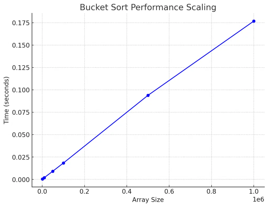
We can see a near-linear relationship between the array size and the time taken, demonstrating Bucket Sort’s efficiency for larger datasets.

Optimizing the Number of Buckets

Optimizing the number of buckets (numBuckets) in Bucket Sort is essential for achieving the best performance. The optimal number of buckets depends on several factors, including the size of the input array and the distribution of the data. Here are a few strategies for determining the optimal number of buckets:

Balance Between Too Few and Too Many Buckets

• Too Few Buckets: If the number of buckets is too small, each bucket will contain too many elements, which will result in more time spent sorting within each bucket. In this case, the advantage of Bucket Sort diminishes as it approaches the performance of traditional sorting algorithms like Quick Sort.
• Too Many Buckets: If the number of buckets is too large, many buckets will be empty or contain very few elements, which adds unnecessary overhead and wastes memory.

Optimal Number of Buckets: O(n)

A general heuristic for the number of buckets is to choose numBuckets proportional to the input size (n). A common rule of thumb is to set the number of buckets equal to the size of the array:

numBuckets= √n

This balances the sorting within each bucket and the overhead of creating and managing the buckets.

Data Distribution Matters

• If the data is uniformly distributed, then a fixed number of buckets works well.
• For non-uniformly distributed data, more complex heuristics may be needed, such as dynamically adjusting the number of buckets based on the data’s range, variance, or clustering characteristics. In these cases, you might use adaptive methods to determine bucket sizes dynamically.

Bucket Load Threshold

Another approach is to keep the number of elements in each bucket roughly equal. You can monitor the load (number of elements) in each bucket and dynamically adjust the number of buckets if some buckets become too full.

Experimentation with Heuristic Tuning

• Start with different values of numBuckets such as n, √n, or multiples of these values.
• Experimentally measure the performance for different input sizes and distributions to find the sweet spot.

Example of Optimizing numBuckets in Code

Here’s an extended version of the Bucket Sort code that allows you to experiment with different values of numBuckets:

#include <iostream>
#include <vector>
#include <algorithm>
#include <ctime>
#include <cstdlib>
#include <chrono>

// Function to implement Bucket Sort
void bucketSort(std::vector<float>& arr, int numBuckets) {
    std::vector<std::vector<float>> buckets(numBuckets);

    for (const float& val : arr) {
        int bucketIndex = numBuckets * val; // Index in range [0, numBuckets-1]
        buckets[bucketIndex].push_back(val);
    }

    for (int i = 0; i < numBuckets; i++) {
        std::sort(buckets[i].begin(), buckets[i].end());
    }

    int index = 0;
    for (int i = 0; i < numBuckets; i++) {
        for (const float& val : buckets[i]) {
            arr[index++] = val;
        }
    }
}

// Function to generate random floating-point numbers
std::vector<float> generateRandomArray(int size) {
    std::vector<float> arr(size);
    for (int i = 0; i < size; i++) {
        arr[i] = static_cast<float>(rand()) / static_cast<float>(RAND_MAX); // Random float [0, 1]
    }
    return arr;
}

// Function to measure performance for different bucket sizes
void measureBucketSortPerformance(int arraySize) {
    std::vector<float> arr = generateRandomArray(arraySize);

    // Experiment with different number of buckets: n, sqrt(n), n/10
    std::vector<int> numBucketsOptions = {arraySize, static_cast<int>(std::sqrt(arraySize)), arraySize / 10};

    for (int numBuckets : numBucketsOptions) {
        auto arrCopy = arr; // Copy the array to avoid side-effects
        auto start = std::chrono::high_resolution_clock::now();
        bucketSort(arrCopy, numBuckets);
        auto end = std::chrono::high_resolution_clock::now();

        std::chrono::duration<double> duration = end - start;
        std::cout << "Array Size: " << arraySize << " | Num Buckets: " << numBuckets 
                  << " | Time: " << duration.count() << " seconds." << std::endl;
    }
}

int main() {
    srand(static_cast<unsigned int>(time(0)));
    int arraySize = 1000000;  // Adjust size as needed

    std::cout << "Performance of Bucket Sort with different numbers of buckets:\n";
    measureBucketSortPerformance(arraySize);

    return 0;
}

Results:

Performance of Bucket Sort with different numbers of buckets:
Array Size: 1000000 | Num Buckets: 1000000 | Time: 1.1496 seconds.
Array Size: 1000000 | Num Buckets: 1000 | Time: 0.218076 seconds.
Array Size: 1000000 | Num Buckets: 100000 | Time: 0.518827 seconds.

Key Insights:

1. Too Many Buckets (1,000,000 Buckets)
   • Time: 1.1496 seconds
   • When the number of buckets equals the size of the array, we observe the worst performance. This is because each bucket contains very few elements, leading to many empty or nearly empty buckets, which introduces overhead.
   • Additionally, creating and managing such a large number of buckets increases the memory usage and the time spent processing and sorting each bucket, even when they are mostly empty.
2. Optimal Buckets (1,000 Buckets)
   • Time: 0.218076 seconds
   • This configuration offers the best performance. The balance between bucket size and the number of elements per bucket is optimal. With 1,000 buckets, each bucket contains enough elements to benefit from the internal sorting step (e.g., std::sort), without having too few or too many elements.
   • Having fewer buckets reduces the overhead of bucket creation and empty bucket management while still allowing the input to be effectively distributed for efficient sorting within each bucket.
3. Moderate Buckets (100,000 Buckets)
   • Time: 0.518827 seconds
   • With 100,000 buckets, performance is better than having 1,000,000 buckets but worse than using 1,000 buckets. While this configuration reduces the empty bucket issue compared to 1,000,000 buckets, there is still some inefficiency due to the smaller number of elements per bucket. Managing such a high number of buckets increases overhead, reducing the sorting efficiency.

Optimal Number of Buckets:

The result suggests that 1,000 buckets is the most optimal choice for an array size of 1,000,000. It provides a good balance between:

• Reducing the number of elements in each bucket, making the internal sorting step fast.
• Avoiding too many buckets that would increase memory overhead and bucket management costs.

Summary

• Too Few Buckets: If the number of buckets is too small (close to 1), the benefit of Bucket Sort is lost as more elements are placed in each bucket, reducing the overall efficiency.
• Too Many Buckets: If there are too many buckets (approaching the array size), you waste time managing empty or near-empty buckets, increasing overhead and slowing down the sort.

The sweet spot for the number of buckets is typically between √n and n/10, depending on the data distribution and array size. For this test with 1,000,000 elements, using 1,000 buckets provided the best performance.

Conclusion

Bucket Sort is a robust non-comparison algorithm that is particularly effective when applied to uniformly distributed datasets across a known range. Its ability to break down sorting into manageable sub-problems (via buckets) allows it to bypass the O (n logn) time complexity lower bound of comparison-based algorithms. This makes it highly efficient for specific use cases, and under the right conditions, it can often outperform traditional comparison-based algorithms like Quick Sort or Merge Sort.

Congratulations on reading to the end of this tutorial!

To implement Bucket Sort in Python, read the article How To Do Bucket Sort in Python.
For further reading on sorting algorithms in C++, go to the articles:

• Shell Sort in C++
• How To Do Quick Sort in C++
• How To Do Selection Sort in C++
• How To Do Comb Sort in C++
• How To Do Insertion Sort in C++

Have fun and happy researching!