How To Do Radix Sort in C++

What is Radix Sort?

Radix Sort is a non-comparative sorting algorithm that sorts numbers by processing individual digits. It sorts the numbers in multiple passes, from the least significant digit (LSD) to the most significant digit (MSD). Radix Sort is particularly effective for sorting integers and is especially useful when dealing with a large volume of data that can fit into the same range.

---

Time Complexity

The time complexity of Radix Sort depends on the number of digits in the maximum number and the number of elements in the array. The complexities are as follows:

• Best Case: O(d * (n + k)), where d is the number of digits in the maximum number, n is the number of elements, and k is the input range.
• Average Case: O(d * (n + k))
• Worst Case: O(d * (n + k))

Space Complexity

The space complexity of Radix Sort is O(n + k), which accounts for the storage of elements in counting arrays used for each digit.

Radix Sort Pseudocode with Explanation

function radixSort(arr):
    maxValue = getMax(arr)                       // Step 1: Find the maximum value in the array
    numDigits = maxDigitLength(maxValue)         // Step 2: Determine the number of digits in the maximum value
    for digitPosition from 1 to numDigits:       // Step 3: Loop through each digit position
        countingSort(arr, digitPosition)         // Step 4: Sort the array based on the current digit

function getMax(arr):
    maxVal = arr[0]
    for each num in arr:
        if num > maxVal:
            maxVal = num
    return maxVal

function maxDigitLength(num):
    count = 0
    while num > 0:
        num = num // 10           // Divide by 10 to remove the last digit
        count += 1                // Increment digit count
    return count

function countingSort(arr, digitPosition):
    const int base = 10
    output = array of size arr.length       // Create an output array to hold the sorted order
    count = array of size base initialized to 0  // Initialize count array for digits 0-9

    // Step 1: Count occurrences of each digit
    for each num in arr:
        index = (num // digitPosition) % base  // Find the digit in the current position
        count[index] += 1                       // Increment the count for this digit

    // Step 2: Change count[i] to contain the actual position of this digit in output[]
    for i from 1 to base - 1:
        count[i] += count[i - 1]               // Cumulative count

    // Step 3: Build the output array
    for i from arr.length - 1 down to 0:       // Process elements in reverse order for stability
        index = (arr[i] // digitPosition) % base
        output[count[index] - 1] = arr[i]      // Place element in its sorted position
        count[index] -= 1                       // Decrement the count for the digit

    // Step 4: Copy the output array back to arr[]
    for i from 0 to arr.length - 1:
        arr[i] = output[i]

Explanation

1. getMax(arr): Finds the maximum value in the array to determine the number of digits.
2. maxDigitLength(maxValue): Calculates the total number of digits in the maximum value.
3. countingSort(arr, digitPosition): Sorts the array based on the current digit using Counting Sort, which is stable and efficient for small ranges.

Radix Sort Implementation in C++

Here is a complete implementation of Radix Sort in C++:

#include <iostream>
#include <vector>
#include <algorithm>

// Function to get the maximum value in the array
int getMax(const std::vector<int>& arr) {
    return *std::max_element(arr.begin(), arr.end());
}

// Counting sort based on the digit at digitPosition
void countingSort(std::vector<int>& arr, int digitPosition) {
    const int base = 10;
    std::vector<int> output(arr.size());
    std::vector<int> count(base, 0);

    // Store count of occurrences in count[]
    for (int num : arr) {
        count[(num / digitPosition) % base]++;
    }

    // Change count[i] to contain the actual position of this digit in output[]
    for (int i = 1; i < base; i++) {
        count[i] += count[i - 1];
    }

    // Build the output array
    for (int i = arr.size() - 1; i >= 0; i--) {
        output[count[(arr[i] / digitPosition) % base] - 1] = arr[i];
        count[(arr[i] / digitPosition) % base]--;
    }

    // Copy the output array to arr[]
    for (int i = 0; i < arr.size(); i++) {
        arr[i] = output[i];
    }
}

// Main radix sort function
void radixSort(std::vector<int>& arr) {
    int maxVal = getMax(arr);
    for (int digitPosition = 1; maxVal / digitPosition > 0; digitPosition *= 10) {
        countingSort(arr, digitPosition);
    }
}

int main() {
    std::vector<int> arr = {170, 45, 75, 90, 802, 24, 2, 66};
    std::cout << "Initial array: ";
    for (int num : arr) {
        std::cout << num << " ";
    }
    radixSort(arr);

    std::cout << "\nSorted array: ";
    for (int num : arr) {
        std::cout << num << " ";
    }
    return 0;
}

Output:

Initial array: 170 45 75 90 802 24 2 66 
Sorted array: 2 24 45 66 75 90 170 802 

Step-by-Step Process of Radix Sort

1. Initial Setup

• Input Array: Start with an unsorted array of integers, e.g., {170, 45, 75, 90, 802, 24, 2, 66}.
• Find Maximum Value: Determine the maximum value in the array using the getMax function. This helps in deciding how many digits the largest number has.

2. Determine the Number of Digits

• Count Digits: Use the maxDigitLength function to find out how many digits are in the maximum value. For example, if the maximum value is 802, it has 3 digits.

3. Sorting by Each Digit

The core of Radix Sort involves sorting the array multiple times based on each digit, from the least significant to the most significant.

First Pass (Least Significant Digit – LSD)

• Digit Position: Start with the least significant digit (1s place).
• Counting Sort: Call the countingSort function to sort the array based on the current digit.
  • Counting Occurrences: Count how many times each digit (0-9) appears at this position.
  • Cumulative Count: Update the count array to determine the position of each digit in the output.
  • Build Output Array: Construct the output array by placing elements in their correct positions based on the digit’s count.
  • Copy to Original Array: Copy the output array back to the original array.

Second Pass (Next Significant Digit – Tens Place)

• Digit Position: Move to the next digit (10s place).
• Counting Sort: Repeat the counting sort process for this digit.
  • Count occurrences for the current digit.
  • Update the cumulative count and build the output array.
  • Copy the output back to the original array.

Third Pass (Most Significant Digit – Hundreds Place)

• Digit Position: Now sort by the most significant digit (100s place).
• Counting Sort: Again, use counting sort for this digit.
  • Count occurrences, update cumulative counts, build the output, and copy it.

4. Final Sorted Array

• Sorted Result: After processing all digit positions, the original array will be sorted. For our example, the final sorted array will be {2, 24, 45, 66, 75, 90, 170, 802}.

Summary of Steps

1. Create Buckets: Initialize the necessary structures for counting occurrences of digits (using a counting array).
2. Distribute Elements: For each digit position, determine which bucket (count index) each element belongs to based on its current digit.
3. Sort Buckets: Sort the elements within each bucket using a stable sorting method (Counting Sort).
4. Concatenate: After sorting each digit, concatenate the sorted buckets to form the original array again, ready for the next digit.
5. Repeat: Continue this process for each digit until all digits have been processed.

Performance test for Radix Sort

Radix Sort is known for its efficiency, particularly when sorting large datasets. Unlike comparison-based sorting algorithms, which have a lower bound of O(n log n) time complexity, Radix Sort can achieve a time complexity of O(d * (n + k)), where:

• d is the number of digits in the maximum number,
• n is the number of elements to be sorted,
• k is the range of the input values.

This makes Radix Sort particularly advantageous when sorting integers or fixed-length strings, especially when the number of digits (d) is significantly smaller than the number of elements (n).

Performance Considerations

In this performance test section, we will analyze how Radix Sort scales with different array sizes and configurations. We will specifically look at:

• Execution Times: By measuring execution times with high precision using the std::chrono library, we can observe how Radix Sort performs across various scenarios—random, sorted, and reverse-sorted arrays.
• Scalability: We will assess how the algorithm handles increasing data and whether its performance aligns with the theoretical time complexity.

#include <iostream>
#include <vector>
#include <algorithm>
#include <chrono>
#include <random>

void countingSort(std::vector<int>& arr, int digitPosition);
void radixSort(std::vector<int>& arr);
int getMax(const std::vector<int>& arr);
int maxDigitLength(int num);
void measureRadixSortPerformance(int arraySize, const std::string& configuration);

// Counting sort based on the digit at digitPosition
void countingSort(std::vector<int>& arr, int digitPosition) {
    const int base = 10;
    std::vector<int> output(arr.size());
    std::vector<int> count(base, 0);

    // Step 1: Count occurrences of each digit
    for (int num : arr) {
        count[(num / digitPosition) % base]++;
    }

    // Step 2: Change count[i] to contain the actual position of this digit in output[]
    for (int i = 1; i < base; i++) {
        count[i] += count[i - 1];
    }

    // Step 3: Build the output array
    for (int i = arr.size() - 1; i >= 0; i--) {
        output[count[(arr[i] / digitPosition) % base] - 1] = arr[i];
        count[(arr[i] / digitPosition) % base]--;
    }

    // Step 4: Copy the output array back to arr[]
    for (int i = 0; i < arr.size(); i++) {
        arr[i] = output[i];
    }
}

// Main radix sort function
void radixSort(std::vector<int>& arr) {
    int maxVal = getMax(arr);
    for (int digitPosition = 1; maxVal / digitPosition > 0; digitPosition *= 10) {
        countingSort(arr, digitPosition);
    }
}

// Function to get the maximum value in the array
int getMax(const std::vector<int>& arr) {
    return *std::max_element(arr.begin(), arr.end());
}

// Function to determine the number of digits in the maximum value
int maxDigitLength(int num) {
    int count = 0;
    while (num > 0) {
        num /= 10;
        count++;
    }
    return count;
}

// Function to generate an array filled with random integers
std::vector<int> generateRandomArray(int size) {
    std::vector<int> arr(size);
    std::mt19937 gen(std::random_device{}()); // Random number generator
    std::uniform_int_distribution<> dis(0, 1000000); // Range of random numbers

    for (int i = 0; i < size; ++i) {
        arr[i] = dis(gen);
    }
    return arr;
}

// Function to generate a sorted array
std::vector<int> generateSortedArray(int size) {
    std::vector<int> arr(size);
    for (int i = 0; i < size; ++i) {
        arr[i] = i; // Sorted array from 0 to size-1
    }
    return arr;
}

// Function to generate a reverse sorted array
std::vector<int> generateReverseSortedArray(int size) {
    std::vector<int> arr(size);
    for (int i = 0; i < size; ++i) {
        arr[i] = size - i - 1; // Reverse sorted array
    }
    return arr;
}

// Function to measure the performance of Radix Sort
void measureRadixSortPerformance(int arraySize, const std::string& configuration) {
    std::vector<int> arr;

    // Generate the array based on the specified configuration
    if (configuration == "random") {
        arr = generateRandomArray(arraySize);
    } else if (configuration == "sorted") {
        arr = generateSortedArray(arraySize);
    } else if (configuration == "reverse_sorted") {
        arr = generateReverseSortedArray(arraySize);
    }

    // Measure execution time
    auto start = std::chrono::high_resolution_clock::now();
    radixSort(arr);
    auto end = std::chrono::high_resolution_clock::now();

    std::chrono::duration<double, std::milli> duration = end - start; // Duration in milliseconds
    std::cout << "Configuration: " << configuration 
              << ", Array Size: " << arraySize 
              << " - Radix Sort took " << duration.count() << " ms." << std::endl;
}

int main() {
    std::vector<int> sizes = {1000, 10000, 100000, 1000000}; // Array sizes to test
    std::vector<std::string> configurations = {"random", "sorted", "reverse_sorted"};

    for (const auto& size : sizes) {
        for (const auto& config : configurations) {
            measureRadixSortPerformance(size, config);
        }
    }

    return 0;
}

Results and Analysis

Configuration	Array Size	Time (ms)
Random	1000	0.456256
Sorted	1000	0.235989
Reverse Sorted	1000	0.233782
Random	10000	4.52651
Sorted	10000	2.9801
Reverse Sorted	10000	2.96853
Random	100000	47.8618
Sorted	100000	34.8683
Reverse Sorted	100000	31.5582
Random	1000000	438.375
Sorted	1000000	375.626
Reverse Sorted	1000000	389.305

Here is the graphical representation of the data:

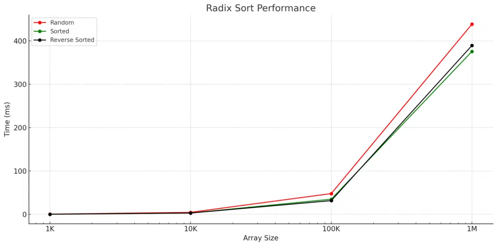
Analysis of the Radix Sort Performance Results

The plot above illustrates the performance of Radix Sort across different array sizes and configurations (random, sorted, and reverse sorted). Here are some key observations and conclusions drawn from the data:

1. Scalability:
   • The execution time increases significantly as the array size grows, consistent with Radix Sort’s expected behavior. This aligns with its theoretical time complexity of O(d * (n + k)), where larger datasets lead to longer sorting times.
2. Configuration Impact:
   • Random Arrays: Radix Sort takes the longest time with random arrays, especially noticeable at larger sizes (e.g., 438.375 ms for 1,000,000 elements). This is expected due to the unpredictability of the digit distributions, which can lead to more sorting passes.
   • Sorted Arrays: The algorithm performs well with already sorted arrays, exhibiting the shortest execution times across all sizes.
   • Reverse-Sorted Arrays: The performance of reverse-sorted arrays is slightly slower than that of sorted arrays but better than that of random arrays. This indicates that while Radix Sort is generally efficient, the initial arrangement of the data still affects its performance.
3. Time Complexity Insights:
   • The differences in execution time highlight the algorithm’s efficiency, particularly in scenarios with sorted or nearly sorted data. The relative constancy of time increases (although exponential) suggests that Radix Sort remains a strong choice for large datasets, especially when the digit length remains manageable.
4. Practical Applications:
   • Given the performance characteristics observed, Radix Sort is particularly suitable for applications that involve sorting integers or fixed-length strings where the input size is large but the digit length is relatively small. For instance, sorting numerical IDs or fixed-length strings in databases would be ideal scenarios for Radix Sort.

Summary of Radix Sort Execution Time Behavior

Execution Time Growth: The overhead from sorting multiple digits results in significant time increases, especially in larger datasets, leading to exponential-like growth in execution time.

Linear Time Complexity: Radix Sort operates with a time complexity of O(d * (n + k)), where d is the number of digits, n is the number of elements, and k is the range of values. Execution time increases linearly with n, influenced by d and k.

Array Size Impact: Larger arrays lead to more comparisons and increased execution time.

Overhead in Each Pass: Each digit processed involves counting sort (O(n + k)), causing cumulative execution time to rise with larger arrays.

Digit Distribution: Non-uniform digit distributions in random arrays can increase the number of operations needed for sorting.

Strengths of Radix Sort

One of Radix Sort’s primary strengths is its ability to sort data in linear time relative to the number of elements, especially when the number of digits in the maximum value is low. Additionally, it is stable, meaning it preserves the relative order of records with equal keys, which can be advantageous in specific applications.

Weaknesses of Radix Sort

It requires additional memory for counting occurrences and can be less efficient for small datasets or data types with large ranges of values. The overhead of processing multiple digits can lead to increased execution time when working with larger numbers or non-integer data types.

When to Use Radix Sort

Radix Sort is well-suited for applications such as sorting numerical data, processing keys in databases, and organizing fixed-length strings in text processing. It excels in scenarios where the dataset is large and the range of values is known, making it an excellent choice for tasks like sorting large lists of IDs or processing large datasets in computational applications.

Conclusion

Radix Sort is a robust non-comparison sorting algorithm that stands out for its efficiency when handling large datasets, particularly those consisting of integers or fixed-length strings. Its time complexity of O(d * (n + k)) allows it to outperform traditional comparison-based algorithms like Quick Sort and Merge Sort in specific scenarios, especially when the range of input values is manageable.

Congratulations on reading to the end of this tutorial!

To implement Radix Sort in Python, read the article How To Do Radix Sort in Python.
For further reading on sorting algorithms in C++, go to the articles:

• Shell Sort in C++
• How To Do Quick Sort in C++
• How To Do Selection Sort in C++
• How To Do Comb Sort in C++
• How To Do Insertion Sort in C++

Have fun and happy researching!