How To Do TimSort in Python

TimSort is a hybrid sorting algorithm that combines Insertion Sort and Merge Sort to deliver efficient performance on real-world data. It was originally designed for Python and is now the default sorting algorithm used by Python’s sorted() function and list.sort(). In this post, we’ll explain how TimSort works, provide a Python implementation, and compare its performance against other sorting algorithms like Quick Sort and Merge Sort.

---

What is TimSort?

TimSort is designed to handle real-world data efficiently by identifying already sorted subsequences, called runs, and merging them. This hybrid approach leverages Insertion Sort for small runs and Merge Sort to combine the runs.

Key Points about TimSort:

• Hybrid Approach: Combines the efficiency of Merge Sort for large datasets and the speed of Insertion Sort for smaller subarrays.
• Runs: TimSort identifies naturally occurring ordered subsequences (runs) and merges them for optimal performance.
• Adaptive: TimSort performs well on partially sorted or nearly sorted data.

---

How TimSort Works

TimSort divides the dataset into small runs and sorts each run using Insertion Sort. It then merges these runs using Merge Sort. The algorithm dynamically adjusts the run size based on the input data.

Steps:

1. Divide the array into runs (typically of size 32 or larger).
2. Sort each run using Insertion Sort.
3. Merge the runs using Merge Sort until the entire array is sorted.

---

TimSort Pseudocode

def timsort(arr):
    min_run = calculate_min_run(len(arr))

    # Sort individual subarrays of size min_run
    for start in range(0, len(arr), min_run):
        insertion_sort(arr, start, min((start + min_run - 1), len(arr) - 1))

    # Start merging the runs
    size = min_run
    while size < len(arr):
        for start in range(0, len(arr), 2 * size):
            mid = start + size - 1
            end = min((start + 2 * size - 1), len(arr) - 1)
            if mid < end:
                merge(arr, start, mid, end)
        size *= 2

• Insertion Sort is used for small chunks (runs).
• Merge Sort is used to combine sorted runs into the final sorted array.

---

Time Complexity of TimSort

• Best Case: O(n) when the input data is already sorted.
• Average Case: O(n log n), as TimSort performs similarly to Merge Sort.
• Worst Case: O(n log n), since even in the worst case, TimSort guarantees efficient sorting.

Space Complexity of TimSort

TimSort requires O(n) additional space to store temporary arrays during the merge phase.

---

Python Implementation of TimSort

import timeit

# Insertion Sort function to sort small runs of the array
def insertion_sort(arr, left, right):
    # Iterate over the array from left + 1 to right
    for i in range(left + 1, right + 1):
        key = arr[i]  # Current element to insert
        j = i - 1  # Previous element index

        # Move elements greater than key one position to the right
        while j >= left and arr[j] > key:
            arr[j + 1] = arr[j]
            j -= 1
        
        # Insert the key element in its correct position
        arr[j + 1] = key

# Merge function to combine two sorted subarrays into one sorted array
def merge(arr, l, m, r):
    # Create temporary arrays to hold the left and right subarrays
    left = arr[l:m + 1]
    right = arr[m + 1:r + 1]
    
    # Indexes for left, right, and main arrays
    i = 0  # Initial index for left subarray
    j = 0  # Initial index for right subarray
    k = l  # Initial index for main array
    
    # Merge the temporary arrays back into arr[l...r]
    while i < len(left) and j < len(right):
        if left[i] <= right[j]:
            arr[k] = left[i]  # Copy smaller element from left subarray
            i += 1
        else:
            arr[k] = right[j]  # Copy smaller element from right subarray
            j += 1
        k += 1

    # Copy any remaining elements from left subarray
    while i < len(left):
        arr[k] = left[i]
        i += 1
        k += 1

    # Copy any remaining elements from right subarray
    while j < len(right):
        arr[k] = right[j]
        j += 1
        k += 1

# Function to calculate the minimum run size for TimSort
# A run is a small portion of the array to be sorted using Insertion Sort
def calculate_min_run(n):
    r = 0  # Used to track if the array size needs to be rounded up
    while n >= 32:
        r |= n & 1  # Keep track of the least significant bit
        n >>= 1  # Divide the array size by 2
    return n + r  # Return the minimum run size (rounded up if necessary)

# Main TimSort function
def timsort(arr):
    n = len(arr)  # Get the size of the array
    min_run = calculate_min_run(n)  # Calculate the minimum run size
    
    # Sort individual subarrays (runs) of size 'min_run' using Insertion Sort
    for start in range(0, n, min_run):
        end = min(start + min_run - 1, n - 1)  # Determine the end of the run
        insertion_sort(arr, start, end)  # Sort the run using Insertion Sort
    
    # Start merging the sorted runs
    size = min_run
    while size < n:
        # Merge pairs of runs of size 'size'
        for left in range(0, n, 2 * size):
            mid = min(n - 1, left + size - 1)  # Calculate the midpoint
            right = min((left + 2 * size - 1), (n - 1))  # Calculate the right end

            # Merge the two runs if there's something to merge
            if mid < right:
                merge(arr, left, mid, right)
        size *= 2  # Double the run size after each pass

# Test array
test_array = [34, 7, 23, 32, 5, 62, 32, 23, 6, 47, 18, 12, 39, 11, 28, 45, 19, 8, 25, 14]

# Function to run TimSort on the array and measure the performance
def run_timsort_performance(arr):
    print("Original array:", arr)  # Print the original unsorted array
    
    # Make a copy of the array and run TimSort
    timsort_arr = arr.copy()
    
    # Measure the execution time of TimSort using timeit
    timsort_time = timeit.timeit(lambda: timsort(timsort_arr), number=1)
    
    # Print the sorted array and the time taken to sort
    print("TimSort result:", timsort_arr)
    print("TimSort execution time (s):", timsort_time)

# Main function to run the performance test
if __name__ == "__main__":
    run_timsort_performance(test_array)  # Run TimSort on the test array

Output:

Original array: [34, 7, 23, 32, 5, 62, 32, 23, 6, 47, 18, 12, 39, 11, 28, 45, 19, 8, 25, 14]
TimSort result: [5, 6, 7, 8, 11, 12, 14, 18, 19, 23, 23, 25, 28, 32, 32, 34, 39, 45, 47, 62]
TimSort execution time (s): 1.600399991730228e-05

Code Explanation

1. insertion_sort:
   • This function sorts small subarrays (runs) of the main array using Insertion Sort, which is efficient for small datasets.
2. merge:
   • Merges two sorted subarrays back into the main array. This is the merging step of TimSort, which combines sorted runs into a larger sorted array.
3. calculate_min_run:
   • Calculates the minimum run size for TimSort, ensuring that the array is divided into appropriately sized subarrays for efficient sorting. A run size of around 32 is common.
4. timsort:
   • This is the main TimSort function. It first divides the array into runs, sorts each run using Insertion Sort, and then merges the sorted runs using the merge function.
5. run_timsort_performance:
   • This function runs TimSort on the test array, prints the original and sorted arrays, and measures the execution time using timeit.
6. Main Block:
   • The if __name__ == "__main__": block ensures that the run_timsort_performance function is executed when the script is run directly.

Walkthrough of TimSort Implementation

Let’s walk through a step-by-step example of how TimSort works with the array used in the code implementation array.

[34, 7, 23, 32, 5, 62, 32, 23, 6, 47, 18, 12, 39, 11, 28, 45, 19, 8, 25, 14]

We will assume that the minimum run size (minRun) is calculated to be 5 for this example. Here’s how TimSort processes the array step-by-step:

Initial Array

[34, 7, 23, 32, 5, 62, 32, 23, 6, 47, 18, 12, 39, 11, 28, 45, 19, 8, 25, 14]

---

Step 1: Divide the Array into Runs

TimSort first breaks the array into runs, each of size minRun = 5. These are the initial runs:

• Run 1: [34, 7, 23, 32, 5]
• Run 2: [62, 32, 23, 6, 47]
• Run 3: [18, 12, 39, 11, 28]
• Run 4: [45, 19, 8, 25, 14]

---

Step 2: Sort Each Run Using Insertion Sort

Now, TimSort applies Insertion Sort to each run to sort it individually.

Sorting Run 1:

• Initial Run: [34, 7, 23, 32, 5]
• Sorted Run: [5, 7, 23, 32, 34]

Sorting Run 2:

• Initial Run: [62, 32, 23, 6, 47]
• Sorted Run: [6, 23, 32, 47, 62]

Sorting Run 3:

• Initial Run: [18, 12, 39, 11, 28]
• Sorted Run: [11, 12, 18, 28, 39]

Sorting Run 4:

• Initial Run: [45, 19, 8, 25, 14]
• Sorted Run: [8, 14, 19, 25, 45]

After sorting, the array looks like this (with each run now sorted):

[5, 7, 23, 32, 34] [6, 23, 32, 47, 62] [11, 12, 18, 28, 39] [8, 14, 19, 25, 45]

---

Step 3: Merge the Runs

After sorting each run, TimSort begins merging them. It merges adjacent runs in pairs using the Merge Sort technique. We merge in multiple passes, doubling the size of the runs with each pass.

First Pass (Merging Runs of Size 5)

Merge Run 1 and Run 2:

• Left Run: [5, 7, 23, 32, 34]
• Right Run: [6, 23, 32, 47, 62]

Merged Run: [5, 6, 7, 23, 23, 32, 32, 34, 47, 62]

Merge Run 3 and Run 4:

• Left Run: [11, 12, 18, 28, 39]
• Right Run: [8, 14, 19, 25, 45]

Merged Run: [8, 11, 12, 14, 18, 19, 25, 28, 39, 45]

After the first pass, the array looks like this:

[5, 6, 7, 23, 23, 32, 32, 34, 47, 62] [8, 11, 12, 14, 18, 19, 25, 28, 39, 45]

---

Second Pass (Merging the Final Two Runs of Size 10)

Now, we merge the two larger runs of size 10:

Merge:

• Left Run: [5, 6, 7, 23, 23, 32, 32, 34, 47, 62]
• Right Run: [8, 11, 12, 14, 18, 19, 25, 28, 39, 45]

Merged Array: [5, 6, 7, 8, 11, 12, 14, 18, 19, 23, 23, 25, 28, 32, 32, 34, 39, 45, 47, 62]

---

Final Sorted Array

After all the runs are merged, we have the fully sorted array:

[5, 6, 7, 8, 11, 12, 14, 18, 19, 23, 23, 25

---

TimSort vs Built-in TimSort vs Merge Sort vs Quick Sort

In Python, sorting efficiency is a critical consideration, especially for larger datasets. TimSort is the default sorting algorithm used by Python’s built-in sorted() and list.sort() functions. It is specifically designed to handle real-world data efficiently by taking advantage of runs (naturally ordered subsequences). But how does it compare with other common sorting algorithms, like Merge Sort and Quick Sort?

In this section, we will compare the performance of:

• TimSort (custom implementation): A hybrid sorting algorithm combining Insertion Sort and Merge Sort.
• Built-in TimSort: The built-in sorted() function, which implements TimSort natively.
• Merge Sort: A stable divide-and-conquer sorting algorithm.
• Quick Sort: A fast, in-place sorting algorithm that, depending on the data, can sometimes outperform others.

We will conduct performance tests on reverse-sorted, random, and sorted arrays of sizes 1000, 5000, 10000, and 50000.

TimSort vs Built-in TimSort vs Merge Sort vs Quick Sort: Performance Test Code

Here is the Python code for the performance test comparison:

import random
import timeit


# TimSort Python implementation
def insertion_sort(arr, left, right):
    for i in range(left + 1, right + 1):
        key = arr[i]
        j = i - 1
        while j >= left and arr[j] > key:
            arr[j + 1] = arr[j]
            j -= 1
        arr[j + 1] = key


def merge(arr, l, m, r):
    left = arr[l:m + 1]
    right = arr[m + 1:r + 1]
    i = 0
    j = 0
    k = l
    while i < len(left) and j < len(right):
        if left[i] <= right[j]:
            arr[k] = left[i]
            i += 1
        else:
            arr[k] = right[j]
            j += 1
        k += 1
    while i < len(left):
        arr[k] = left[i]
        i += 1
        k += 1
    while j < len(right):
        arr[k] = right[j]
        j += 1
        k += 1


def calculate_min_run(n):
    r = 0
    while n >= 32:
        r |= n & 1
        n >>= 1
    return n + r


def timsort(arr):
    n = len(arr)
    min_run = calculate_min_run(n)
    for start in range(0, n, min_run):
        end = min(start + min_run - 1, n - 1)
        insertion_sort(arr, start, end)
    size = min_run
    while size < n:
        for left in range(0, n, 2 * size):
            mid = min(n - 1, left + size - 1)
            right = min((left + 2 * size - 1), (n - 1))
            if mid < right:
                merge(arr, left, mid, right)
        size *= 2


# Merge Sort Python implementation
def merge_sort(arr):
    if len(arr) > 1:
        mid = len(arr) // 2
        left = arr[:mid]
        right = arr[mid:]
        merge_sort(left)
        merge_sort(right)
        i = j = k = 0
        while i < len(left) and j < len(right):
            if left[i] < right[j]:
                arr[k] = left[i]
                i += 1
            else:
                arr[k] = right[j]
                j += 1
            k += 1
        while i < len(left):
            arr[k] = left[i]
            i += 1
            k += 1
        while j < len(right):
            arr[k] = right[j]
            j += 1
            k += 1


# Quick Sort Python implementation
def quick_sort(arr):
    if len(arr) <= 1:
        return arr
    pivot = arr[len(arr) // 2]
    left = [x for x in arr if x < pivot]
    middle = [x for x in arr if x == pivot]
    right = [x for x in arr if x > pivot]
    return quick_sort(left) + middle + quick_sort(right)


# Test arrays and sizes
array_sizes = [1000, 5000, 10000, 50000]


# Function to generate different array types
def generate_random_array(size):
    return [random.randint(0, 100000) for _ in range(size)]


def generate_sorted_array(size):
    return list(range(size))


def generate_reverse_sorted_array(size):
    return list(range(size, 0, -1))


# Performance test function
def run_performance_test():
    for size in array_sizes:
        # Generate test arrays
        random_array = generate_random_array(size)
        sorted_array = generate_sorted_array(size)
        reverse_sorted_array = generate_reverse_sorted_array(size)

        # Measure TimSort performance
        timsort_time_random = timeit.timeit(lambda: timsort(random_array.copy()), number=1)
        timsort_time_sorted = timeit.timeit(lambda: timsort(sorted_array.copy()), number=1)
        timsort_time_reverse = timeit.timeit(lambda: timsort(reverse_sorted_array.copy()), number=1)

        # Measure built-in TimSort performance
        builtin_time_random = timeit.timeit(lambda: sorted(random_array.copy()), number=1)
        builtin_time_sorted = timeit.timeit(lambda: sorted(sorted_array.copy()), number=1)
        builtin_time_reverse = timeit.timeit(lambda: sorted(reverse_sorted_array.copy()), number=1)

        # Measure Merge Sort performance
        merge_time_random = timeit.timeit(lambda: merge_sort(random_array.copy()), number=1)
        merge_time_sorted = timeit.timeit(lambda: merge_sort(sorted_array.copy()), number=1)
        merge_time_reverse = timeit.timeit(lambda: merge_sort(reverse_sorted_array.copy()), number=1)

        # Measure Quick Sort performance
        quick_time_random = timeit.timeit(lambda: quick_sort(random_array.copy()), number=1)
        quick_time_sorted = timeit.timeit(lambda: quick_sort(sorted_array.copy()), number=1)
        quick_time_reverse = timeit.timeit(lambda: quick_sort(reverse_sorted_array.copy()), number=1)

        # Print results for current size
        print(f"\nArray Size: {size}")
        print(f"TimSort Random: {timsort_time_random}, Sorted: {timsort_time_sorted}, Reverse: {timsort_time_reverse}")
        print(
            f"Built-in TimSort Random: {builtin_time_random}, Sorted: {builtin_time_sorted}, Reverse: {builtin_time_reverse}")
        print(f"Merge Sort Random: {merge_time_random}, Sorted: {merge_time_sorted}, Reverse: {merge_time_reverse}")
        print(f"Quick Sort Random: {quick_time_random}, Sorted: {quick_time_sorted}, Reverse: {quick_time_reverse}")


if __name__ == "__main__":
    run_performance_test()

Output:

Array Size: 1000
TimSort Random: 0.0016450809998787008, Sorted: 0.0007437870008288883, Reverse: 0.0022481460000562947
Built-in TimSort Random: 0.00011601100050029345, Sorted: 1.3477001630235463e-05, Reverse: 1.3111999578541145e-05
Merge Sort Random: 0.0017311960000370163, Sorted: 0.0015043709972815122, Reverse: 0.0014318670000648126
Quick Sort Random: 0.0014248229999793693, Sorted: 0.0009857160002866294, Reverse: 0.0009490580014244188

Array Size: 5000
TimSort Random: 0.009803203000046778, Sorted: 0.005523790998267941, Reverse: 0.009131142000114778
Built-in TimSort Random: 0.0005888630003028084, Sorted: 5.1107999752275646e-05, Reverse: 4.8904999857768416e-05
Merge Sort Random: 0.009586225001839921, Sorted: 0.007666212997719413, Reverse: 0.007884531001764117
Quick Sort Random: 0.007720534998952644, Sorted: 0.005034844001784222, Reverse: 0.0053981370001565665

Array Size: 10000
TimSort Random: 0.018811097001162125, Sorted: 0.011846479999803705, Reverse: 0.01917889899777947
Built-in TimSort Random: 0.0013478220025717746, Sorted: 0.00011578900011954829, Reverse: 0.000139667001349153
Merge Sort Random: 0.02028500999949756, Sorted: 0.016429164999863133, Reverse: 0.016625714000838343
Quick Sort Random: 0.01639097000224865, Sorted: 0.011415228000259958, Reverse: 0.011007416000211379

Array Size: 50000
TimSort Random: 0.11906276800073101, Sorted: 0.07946215400079382, Reverse: 0.1282699010007491
Built-in TimSort Random: 0.007791060997988097, Sorted: 0.0005915309993724804, Reverse: 0.0005682640003215056
Merge Sort Random: 0.12111129199911375, Sorted: 0.09526197599916486, Reverse: 0.09691753899824107
Quick Sort Random: 0.08853945900045801, Sorted: 0.060585850002098596, Reverse: 0.06230688100185944

Let’s put these results together in several line plots and analyse them.

# Plotting the results with specific colors for the lines: red, blue, green, and black
plt.figure(figsize=(14, 10))

# Plot for Random arrays
plt.subplot(3, 1, 1)
plt.plot(df['Array Size'], df['TimSort Random'], label="TimSort", marker='o', color='red')
plt.plot(df['Array Size'], df['Built-in TimSort Random'], label="Built-in TimSort", marker='o', color='blue')
plt.plot(df['Array Size'], df['Merge Sort Random'], label="Merge Sort", marker='o', color='green')
plt.plot(df['Array Size'], df['Quick Sort Random'], label="Quick Sort", marker='o', color='black')
plt.title('Performance on Random Arrays')
plt.xlabel('Array Size')
plt.ylabel('Time (s)')
plt.xscale('log')
plt.legend()

# Plot for Sorted arrays
plt.subplot(3, 1, 2)
plt.plot(df['Array Size'], df['TimSort Sorted'], label="TimSort", marker='o', color='red')
plt.plot(df['Array Size'], df['Built-in TimSort Sorted'], label="Built-in TimSort", marker='o', color='blue')
plt.plot(df['Array Size'], df['Merge Sort Sorted'], label="Merge Sort", marker='o', color='green')
plt.plot(df['Array Size'], df['Quick Sort Sorted'], label="Quick Sort", marker='o', color='black')
plt.title('Performance on Sorted Arrays')
plt.xlabel('Array Size')
plt.ylabel('Time (s)')
plt.xscale('log')
plt.legend()

# Plot for Reverse Sorted arrays
plt.subplot(3, 1, 3)
plt.plot(df['Array Size'], df['TimSort Reverse'], label="TimSort", marker='o', color='red')
plt.plot(df['Array Size'], df['Built-in TimSort Reverse'], label="Built-in TimSort", marker='o', color='blue')
plt.plot(df['Array Size'], df['Merge Sort Reverse'], label="Merge Sort", marker='o', color='green')
plt.plot(df['Array Size'], df['Quick Sort Reverse'], label="Quick Sort", marker='o', color='black')
plt.title('Performance on Reverse Sorted Arrays')
plt.xlabel('Array Size')
plt.ylabel('Time (s)')
plt.xscale('log')
plt.legend()

plt.tight_layout()
plt.show()

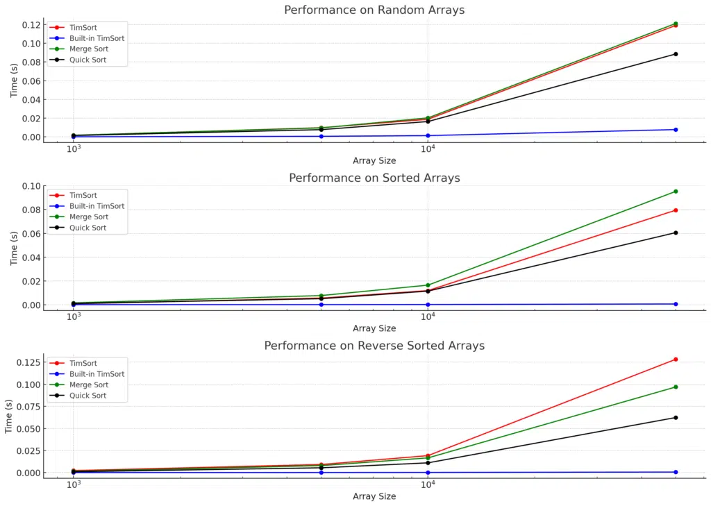
Analysis of the Results

Based on the results plotted for TimSort, Built-in TimSort, Merge Sort, and Quick Sort across varying array sizes (1000, 5000, 10000, 50000) for random, sorted, and reverse-sorted arrays, here are the key insights:

1. Performance on Random Arrays

• Built-in TimSort consistently outperforms all other algorithms on random arrays, showing the lowest execution time for all array sizes. This is expected since Python’s built-in sorted() function is highly optimized for real-world data.
• Quick Sort performs better than both TimSort (custom implementation) and Merge Sort as the array size increases, especially at sizes 10000 and 50000.
• TimSort (custom) and Merge Sort perform comparably for smaller arrays, but Merge Sort tends to be slightly slower for larger arrays (10000, 50000). However, the differences are not substantial.

2. Performance on Sorted Arrays

• Built-in TimSort performs exceptionally well, with near-instantaneous execution times, demonstrating its adaptability to already sorted data.
• Quick Sort suffers on sorted arrays because of its poor pivot selection, leading to comparatively slower execution. However, it still improves significantly for larger arrays compared to its performance on reverse-sorted arrays.
• Custom TimSort shows moderate improvement in performance over random arrays but is still slower than Built-in TimSort, particularly for larger arrays (50000).
• Merge Sort shows slightly better performance on sorted arrays than random or reverse-sorted data but still lags behind TimSort and Quick Sort.

3. Performance on Reverse-Sorted Arrays

• Built-in TimSort continues to dominate, handling reverse-sorted data with minimal overhead, as it’s designed to handle disorder efficiently.
• Quick Sort shows worse performance on reverse-sorted arrays, especially as the array size grows, due to its reliance on pivots, which leads to inefficient partitioning.
• Custom TimSort and Merge Sort show consistent execution times, with Merge Sort slightly outperforming TimSort in larger datasets.

---

Key Takeaways

1. Built-in TimSort (Python’s sorted()) is the clear winner across all dataset types (random, sorted, and reverse). Its optimized implementation allows it to efficiently handle even large datasets, with near-instantaneous results on sorted and reverse-sorted data.
2. Custom TimSort performs decently but is generally slower than Built-in TimSort. It performs similarly to Merge Sort but isn’t as optimized for sorted or reverse-sorted data.
3. Quick Sort is generally faster than TimSort and Merge Sort for random datasets but struggles with sorted and reverse-sorted data due to its pivot selection strategy, leading to higher execution times.
4. Merge Sort is stable across all dataset types, offering consistent performance, though it tends to be slower than both Quick Sort and TimSort for random and sorted arrays.

We have considered random, reverse-sorted and sorted, but what happens when we use partially sorted data?

First, let’s update the code with a function to generate partially sorted data and a function to run test. Then, in the main function we will add the new test to run.

import random
import timeit

# Function to generate a partially sorted array
def generate_partially_sorted_array(size, sorted_ratio=0.8):
    # Create the sorted part
    sorted_part = list(range(int(size * sorted_ratio)))
    # Create the random part
    random_part = [random.randint(0, 100000) for _ in range(size - int(size * sorted_ratio))]
    # Combine the sorted and random parts
    return sorted_part + random_part

# TimSort, Merge Sort, and Quick Sort implementations remain the same

# Performance test function for partially sorted data
def run_partial_sort_test():
    array_sizes = [1000, 5000, 10000, 50000]
    
    for size in array_sizes:
        # Generate a partially sorted array
        partial_array = generate_partially_sorted_array(size)

        # Measure TimSort performance
        timsort_time = timeit.timeit(lambda: timsort(partial_array.copy()), number=1)

        # Measure built-in TimSort performance
        builtin_time = timeit.timeit(lambda: sorted(partial_array.copy()), number=1)

        # Measure Merge Sort performance
        merge_time = timeit.timeit(lambda: merge_sort(partial_array.copy()), number=1)

        # Measure Quick Sort performance
        quick_time = timeit.timeit(lambda: quick_sort(partial_array.copy()), number=1)

        # Print results for current size
        print(f"\nArray Size: {size}")
        print(f"TimSort: {timsort_time}")
        print(f"Built-in TimSort: {builtin_time}")
        print(f"Merge Sort: {merge_time}")
        print(f"Quick Sort: {quick_time}")

if __name__ == "__main__":
    run_partial_sort_test()

Remember: we have defined TimSort, Merge Sort and Quick Sort in the earlier section.

Output:

Array Size: 1000
TimSort: 0.0009682749987405259
Built-in TimSort: 3.115900108241476e-05
Merge Sort: 0.0015091430032043718
Quick Sort: 0.0010818410009960644

Array Size: 5000
TimSort: 0.007126232001610333
Built-in TimSort: 0.00020182600201223977
Merge Sort: 0.009563522999087581
Quick Sort: 0.006542889001138974

Array Size: 10000
TimSort: 0.013235039998107823
Built-in TimSort: 0.0002871409997169394
Merge Sort: 0.01710491300036665
Quick Sort: 0.011640069002169184

Array Size: 50000
TimSort: 0.0786541989982652
Built-in TimSort: 0.001943560997460736
Merge Sort: 0.10525926599802915
Quick Sort: 0.07033605399919907

On a graph, the numbers look like this:

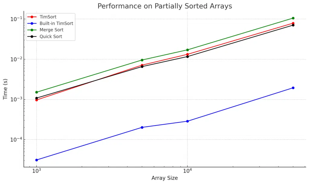
Analysis of the Performance on Partially Sorted Data

From the results, we can observe how TimSort, Built-in TimSort, Merge Sort, and Quick Sort perform on partially sorted arrays across different sizes.

Performance Breakdown:

1. Built-in TimSort:
   • Performance: The built-in TimSort is significantly faster than the custom implementations of all other algorithms across all array sizes.
   • Reason: This is because Python’s built-in sorted() is highly optimized for real-world datasets, including partially sorted arrays. It identifies runs and minimizes unnecessary operations, taking full advantage of the existing order in the data.
2. Custom TimSort:
   • Performance: The custom TimSort performs reasonably well but is slower than the Built-in TimSort and slightly slower than Quick Sort in most cases.
   • Reason: Although TimSort is designed to handle partially sorted data, the overhead of run detection and merging operations in the custom implementation introduces more overhead compared to the highly optimized built-in version.
3. Merge Sort:
   • Performance: Merge Sort consistently shows slower performance than both TimSort and Quick Sort for partially sorted data.
   • Reason: Merge Sort does not take advantage of pre-existing order in the data. It follows a strict divide-and-conquer approach, recursively splitting the data in half and merging, which leads to redundant comparisons and operations on already sorted data.
4. Quick Sort:
   • Performance: Quick Sort generally performs faster than Merge Sort and is competitive with TimSort.
   • Reason: While Quick Sort’s performance doesn’t degrade as much on partially sorted data as it does on fully sorted or reverse-sorted data, it still doesn’t take full advantage of existing order, unlike TimSort.

Key Takeaways:

• Built-in TimSort excels in handling partially sorted data, leveraging optimizations such as detecting runs and minimizing operations on sorted sequences. Its performance is much faster compared to the other algorithms, with near-instantaneous sorting for smaller arrays.
• Custom TimSort performs decently on partially sorted data but is slower than Quick Sort and Built-in TimSort due to its hybrid nature and extra overhead in managing runs and merging.
• Quick Sort continues to be competitive but doesn’t adapt to the partial order in the data as efficiently as TimSort, making it slower than both the built-in version and custom TimSort.
• Merge Sort does not optimize for pre-existing order, resulting in the slowest performance on partially sorted data.

Why is the Built-in TimSort the Best?

1. Highly Optimized Code:

• The built-in sorted() and list.sort() functions in Python have been optimized at a low level in the C programming language. This allows the built-in TimSort to leverage highly efficient memory management, faster operations, and better CPU usage compared to custom implementations written in Python, which are generally slower due to Python’s higher-level nature and lack of the same optimization opportunities.

2. Efficient Memory Management:

• The built-in TimSort is implemented in C, which allows it to manage memory more efficiently. It avoids unnecessary memory allocations and deallocations that might occur in a custom Python implementation. This gives the built-in version an edge in speed, especially for larger datasets.

3. Adaptive Improvements:

• Python’s built-in TimSort includes numerous adaptive features beyond the basic algorithm, such as identifying and skipping already sorted runs. These optimizations allow it to minimize work when sorting data with patterns of partial order, making it extremely fast for real-world datasets that are often not fully randomized.
• In contrast, custom implementations may lack these sophisticated optimizations and thus perform more comparisons or unnecessary operations.

4. Better Cache Utilization:

• The built-in TimSort is designed to efficiently use the CPU cache, which reduces cache misses and improves overall sorting speed. The custom implementation in Python does not take full advantage of cache optimization, leading to slower performance when dealing with larger datasets.

5. Low-Level Optimizations:

• The C implementation of the built-in sort benefits from a range of low-level optimizations, such as avoiding function calls within tight loops, which makes the execution faster. Additionally, Python’s sorted() function avoids some of the overhead of interpreted Python code, further improving its performance.

6. Algorithmic Tweaks:

• The built-in TimSort incorporates additional tweaks to improve performance in edge cases, such as choosing the right pivot size for merging runs, reducing the overhead of the merge step, and dynamically adjusting the minimum run size for certain datasets. These tweaks are often overlooked or not fully implemented in custom versions.

7. Tested and Refined:

• Python’s built-in TimSort has undergone extensive testing, refinement, and optimization over many years. It is designed for correctness and efficiency and has been fine-tuned to work well for a wide range of input types and sizes.
• While functional, a custom implementation is unlikely to undergo the same level of testing and refinement and may, therefore, lack these optimizations and reliability.

---

Advantages of TimSort

• Efficient for real-world data: Handles partially sorted data better than traditional algorithms like Quick Sort.
• Stable: Maintains the relative order of equal elements, making it suitable for multi-criteria sorting.
• Fast for Small Datasets: Uses Insertion Sort for small runs, which is fast for small or partially sorted arrays.

---

Limitations of TimSort

• Memory Usage: Requires O(n) extra space due to its reliance on merging runs.
• Not Ideal for Random Data: While TimSort is fast, it doesn’t outperform Quick Sort on completely random data.

---

When to Use TimSort

TimSort is ideal for applications where:

• Partial Ordering: The dataset contains partially sorted or nearly sorted sequences.
• Stability Matters: Situations where maintaining the relative order of equal elements is important.
• Real-World Data: TimSort is designed to handle real-world data patterns efficiently, making it the default sorting algorithm in Python.

---

Differences in Implementing TimSort in Python vs. C++

1. Performance Overhead:
   • Python: Python is an interpreted language, and its dynamic nature introduces significant overhead during execution. Each function call, memory allocation, and loop iteration is slower in Python compared to C++ due to the interpreter overhead.
   • C++: In contrast, C++ is a compiled language. When implemented in C++, TimSort can use compiler optimizations like inlining, aggressive loop unrolling, and efficient memory management, making the algorithm run faster with less overhead.
2. Memory Management:
   • Python: Memory management in Python is automatic (via garbage collection), which can introduce inefficiencies. The cost of memory allocations and deallocations is higher in Python, particularly for temporary arrays used during merging.
   • C++: In C++, memory management can be handled more precisely using manual allocation, stack allocation, or more efficient data structures. This leads to faster and more predictable memory usage during sorting operations, especially in TimSort, where runs are continuously merged.
3. Lower-level Control:
   • C++: Provides lower-level control over the hardware, such as better cache utilization, direct memory access, and fewer abstractions between the code and machine. This can significantly boost the performance of an algorithm like TimSort, which frequently interacts with memory.
   • Python: Lacks this level of control, which means it cannot fully take advantage of the hardware’s capabilities, resulting in slower performance for memory-intensive operations like merging runs.
4. Multi-threading and Parallelism:
   • C++: It’s easier to implement parallelism in C++ to boost performance for large datasets. TimSort in C++ could be parallelized to handle different runs or merge processes concurrently.
   • Python: Python’s Global Interpreter Lock (GIL) limits true multi-threaded execution, making it harder to maximally exploit parallelism in a custom TimSort implementation.

Conclusion

TimSort offers an adaptive, stable, efficient sorting solution for many real-world applications. It outperforms algorithms like Quick Sort and Merge Sort when handling partially sorted data. Its combination of Insertion Sort and Merge Sort ensures optimal performance across various input types. Although it may not always be the fastest for completely random data, its adaptability makes it a versatile tool for general-purpose sorting in Python.

Congratulations on reading to the end of this tutorial!

To implement TimSort in C++, go to the article How To Do TimSort in C++.

• How to do Insertion Sort in Python
• How to Do Bubble Sort in Python
• How to do Quick Sort in Python
• How to do Merge Sort in Python
• How to do Counting Sort in Python
• How to Do Radix Sort in Python
• How to Do Bucket Sort in Python
• How to Do Pigeonhole Sort in Python
• How To Do Comb Sort in Python 
• How to Do Shell Sort in Python

Have fun and happy researching!