Implied volatility tells us the expected volatility of a stock over an option’s lifetime. Implied volatility is directly influenced by the supply and demand of the options and the market’s expectation of the direction of the price of the underlying security. As expectations rise or the demand for an option increases, implied volatility will increase. As implied volatility increases, the option price increases.
On the other hand, as the market’s expectations decrease or the demand for an option falls, implied volatility will also fall. As implied volatility decreases, the option price decreases.
This tutorial will go through an option’s implied volatility and how to calculate it with C++. We will consider root-finding methods to calculate implied volatility: Newton-Raphson, Interval Bisection, and Brute Force.
Table of contents
What is Implied Volatility?
Before going through implied volatility, you should have gone through the Black-Scholes formula and the Options Greeks.
We can use the Black-Scholes Formula to price a European option. We need five variables: stock price, exercise price, time to expiration, risk-free interest rate, and standard deviation of log returns or volatility. Let’s look at a diagram describing a European call option.
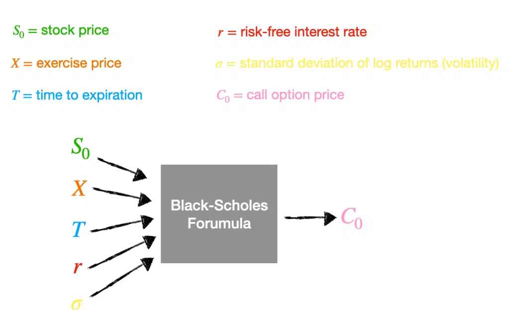
The first four variables are easy to find. We can easily find the stock price. The exercise price is part of the contract. We can approximate the risk-free interest rate by assuming it equals the interest rate on a three-month government Treasury bill. The time to expiration we can calculate using today’s date and when the contract will expire. However, volatility is tricky; it is not a constant value.
We can estimate the volatility of an option by looking at the history of the standard deviation of log returns.
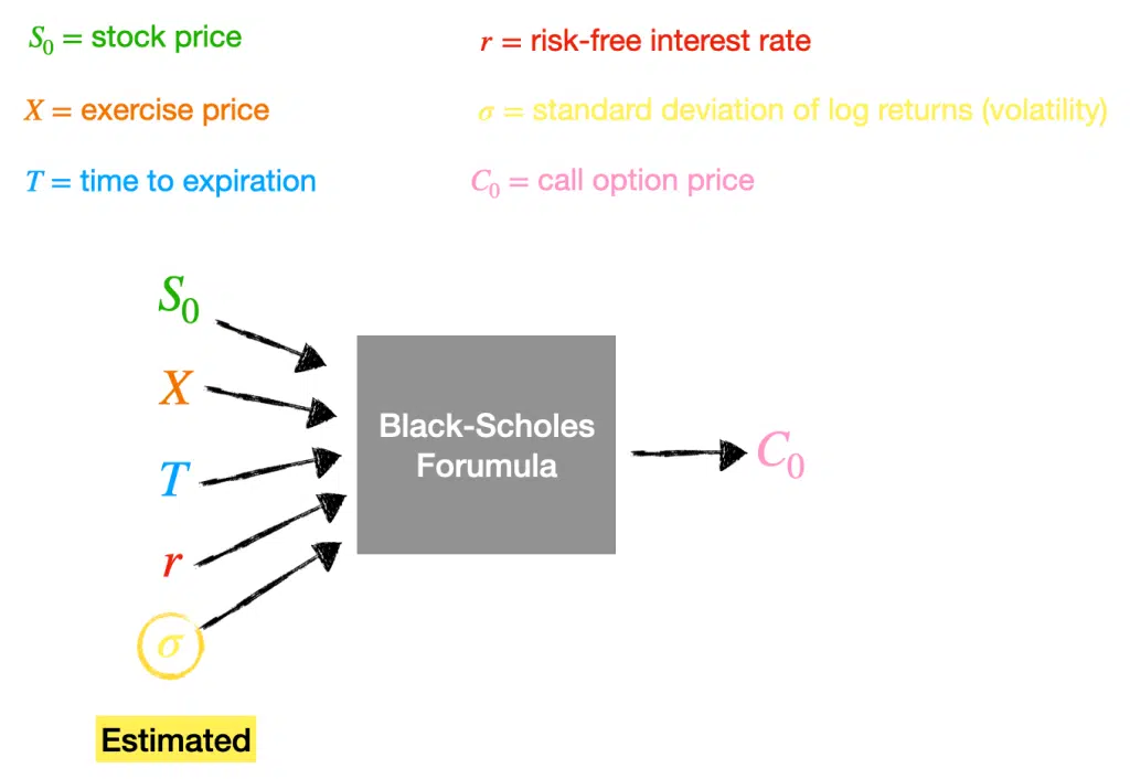
Any volatility value is an estimate, and there is an assumption that this variable will be constant over the option’s lifetime.
However, options are traded constantly, and we can look up the market price for a call option for a given stock price, exercise price, risk-free interest rate and time to expiration.
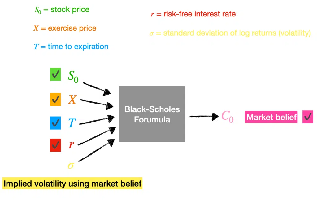
Suppose we know the market price or what the market believes the option price should be based on transactions and known variables. In that case, we can work backwards through Black-Scholes to determine the market estimate for the volatility or implied volatility.
If the market gets more unpredictable, the market will pay more for a given option, driving the implied volatility up. We can aggregate the implied volatility across multiple securities to find implied volatility for given markets at a time.
Remember, the implied volatility depends on an option’s market price, not the other way around.
Let’s look at the Black-Scholes formula for pricing a European call option:
$$C= S_{0}N(d_{1})~- Xe^{-r\tau}N(d_{2}) $$
where,
$$d_{1} = \frac{\text{ln}\frac{S_{0}}{X} + (r + \sigma^{2}/2)*\tau}{\sigma\sqrt{\tau}}, \qquad d_{2} = \frac{\text{ln}\frac{S_{0}}{X} + (r – \sigma^{2}/2)*\tau}{\sigma\sqrt{\tau}} = d_{1} – \sigma\sqrt{\tau}$$
- S: current underlying price
- K: strike price of option
- r: risk-free interest rate
- T: time until option expiration
- $\sigma: ~\text{annual volatility of underlying security’s returns}$
- N(x): cumulative distribution function for a standard normal distribution
Let’s say we want to find the implied volatility for an option with a current price for the underlying at \$100 for the right to buy the stock a year from the current date for \$125. The call option costs \$25, and the risk-free interest rate is 5%. If we put all of these values in the Black-Scholes formula, we will get the following:
$$25= 100 * N(\frac{\text{ln}\frac{100}{125} + (0.05 + \sigma^{2}/2)*1}{\sigma\sqrt{1}})~- 125e^{-0.05*1}N(\frac{\text{ln}\frac{100}{125} + (0.05 – \sigma^{2}/2)*1}{\sigma\sqrt{1}} $$
The unknown value in this equation is the volatility. We need to solve for volatility in the equation to return a call price of $18. We can solve this equation using iterative methods.
Now let’s look at the iterative methods to find the implied volatility in C++.
Implied volatility using Newton Raphson Method
The first method we will look at is the Newton-Raphson method. The Newton-Raphson method is a way to quickly find an approximation for the root of a real-valued function. The method considers that a straight-line tangent can approximate a continuous and differentiable function.
Newton Raphson Algorithm
- $\text{Define a continuous, differentiable function}~ f(x)$
- $\text{Take an initial guess for the root}~ x = x_{0},~\text{approximate the root guess with}~ x_{1} = \frac{f(x_{0})}{f'(x_{0})}.$
- $\text{Iterate as follows:}~ x_{n+1} = x_{n} – \frac{f(x_{n})}{f'(x_{n})}$
- $\text{Break if}~ |f(x_{n})| < \epsilon.~ \text{Where}~ \epsilon ~\text{is the tolerance for error}.$
When we apply the Newton-Raphson Algorithm to solve for implied volatility, we get the following:
- $\text{Our continuous, differentiable function is: }~f(\sigma) = V_{BS_{\sigma}} – V_{market}$
- $\text{Our initial guess is}~\sigma_{0} = 0.30$
- $\text{Iterate as follows:}~ \sigma_{n+1} = \sigma_{n} – \frac{V_{BS_{\sigma}} – V_{market}}{\frac{\partial V_{BS_{\sigma}}}{\partial \sigma}}$
- $\text{Break if}~ |V_{BS_{\sigma}} – V_{market}| < \epsilon,~ \text{return}~ \sigma_{n}.$
C++ Code for Newton Raphson
First, we will define the normal probability density function, cumulative distribution function, and the d1 and d2 variables. We will save this code in a file called bs_prices.h.
#ifndef IMPLIED_VOLATILITY_BS_PRICES_H
#define IMPLIED_VOLATILITY_BS_PRICES_H

#define _USE_MATH_DEFINES
#include <iostream>
#include <cmath>

// Standard normal probability density function
double norm_pdf(const double& x) {
    return (1.0/(pow(2*M_PI,0.5)))*exp(-0.5*x*x);
}
// Standard cumulative distribution function

double norm_cdf(const double x){
        return std::erfc(-x/std::sqrt(2))/2;
    }

// Define functions for d_1 and d_2

double d_1(const double& S, const double& K, const double& r, const double& T, const double& sig){
    return  (log(S/K) + (r + pow(sig,2)/2)*T) / (sig*(pow(T,0.5)));
}

double d_2(const double& S, const double& K, const double& r, const double& T, const double& sig) {
    return (log(S/K) + (r - pow(sig,2)/2)*T) / (sig*(pow(T,0.5)));
}
Next, we will define the functions for pricing a call or put option using the Black-Scholes formula and a function for calculating the vega of an option. We will also save this code in the file bs_prices.h.
// Calculate the European vanilla call price based on
// underlying S, strike K, risk-free rate r, volatility of
// underlying sigma and time to maturity T

double call_price(const double& S, const double& K, const double& r, const double& T, const double& sig) {
    return S * norm_cdf((d_1(S, K, r, T, sig))) - K*exp(-r * T) * norm_cdf(d_2(S,K, r, T, sig));
}

double put_price(const double& S, const double& K, const double& r, const double& T, const double& sig) {
    return -S * norm_cdf(-d_1(S, K, r, T, sig)) + K*exp(-r*T)* norm_cdf(-d_2(S,K, r, T, sig));
}

double vega(const double& S, const double& K, const double& r, const double& T, const double& sig) {
    return S * sqrt(T) * norm_pdf((d_1(S, K, r, T, sig)));
}

double black_scholes_func(const double& S, const double& K, const double& r, const double& T, const double& sig, const bool& cp) {
    if (cp){
        return call_price(S, K, r, T, sig);
    } else {
        return put_price(S, K, r, T, sig);
    }
}
Now we can put it all together and find the implied volatility using the Newton-Raphson algorithm in bs_prices.h:
// Calculate the European vanilla call/put option implied volatility
// Using Newton-Raphson root finding method

double implied_volatility_nr(const double& C_M, const double& S, const double& K, const double& r, const double& T, const bool& cp, const double& tol, const double& max_iterations) {
    double sigma = 0.3;

    for (int i =0; i < max_iterations; i++){

        double market_price = black_scholes_func(S, K, r, T, sigma, cp);

        double diff = market_price - C_M;


        if (abs(diff) < tol)

            break;

        else

            sigma = sigma - diff / vega(S, K, r, T, sigma);

    }

    return sigma * 100;
}
#endif //IMPLIED_VOLATILITY_BS_PRICES_H
Let’s test the code for a call option in our main program:
#ifndef IMPLIED_VOLATILITY_BLACK_SCHOLES_CPP
#define IMPLIED_VOLATILITY_BLACK_SCHOLES_CPP

#include "bs_prices.h"
#include <iostream>

int main() {
double S = 100.0;
double K = 125.0;
double r = 0.05;
double T = 1.0;
// Market belief price
double C_M =25;

double epsilon = 0.0001;
double sigma_nr = implied_volatility_nr(C_M, S, K, r, T, true, epsilon, 100);
std::cout << "Implied Volatility using newton raphson:  " << sigma_nr << "%" << std::endl;
return 0;
}

#endif
Implied Volatility using newton raphson: 79.1834%
We found the implied volatility for the call option to be 79.18%.
If we plug the implied volatility value into the Black-Scholes formula, we will get the market price for the call option.
#ifndef IMPLIED_VOLATILITY_BLACK_SCHOLES_CPP
#define IMPLIED_VOLATILITY_BLACK_SCHOLES_CPP

#include "bs_prices.h"
#include <iostream>

int main() {
double S = 100.0;
double K = 125.0;
double r = 0.05;
double T = 1.0;
// Market belief price
double C_M =25;

double epsilon = 0.0001;
double sigma_nr = implied_volatility_nr(C_M, S, K, r, T, true, epsilon, 100);
double price = black_scholes_func(S, K, r, T, sigma_nr/100, true);
std::cout << "Implied Volatility using newton raphson:  " << sigma_nr << "%" << std::endl;
std::cout << "Call price using implied volatility:  $" << price <<std::endl;

return 0;
}

#endif
Implied Volatility using newton raphson:  79.1834%
Call price using implied volatility:  $25
Let’s test the code for a put option:
#ifndef IMPLIED_VOLATILITY_BLACK_SCHOLES_CPP
#define IMPLIED_VOLATILITY_BLACK_SCHOLES_CPP

#include "bs_prices.h"
#include <iostream>

int main() {
double S = 100.0;
double K = 125.0;
double r = 0.05;
double T = 1.0;
// Market belief price
double C_M =25;

double epsilon = 0.0001;
double sigma_nr = implied_volatility_nr(C_M, S, K, r, T, false, epsilon, 100);
double price = black_scholes_func(S, K, r, T, sigma_nr/100, false);

std::cout << "Implied Volatility using newton raphson:  " << sigma_nr << "%" << std::endl;
std::cout << "Put price using implied volatility:  $" << price <<std::endl;

return 0;
}

#endif
Implied Volatility using newton raphson:  31.1055%
Price using implied volatility:  $25
We found the implied volatility for the put option to be 31.11%. When we plug the implied volatility value into the Black-Scholes formula, we get the market price for the put option of $25.
Implied Volatility Using Bisection Method
The second method we will look at is the Interval Bisection method. The interval bisection method does not require numerical derivatives to calculate the implied volatility.
Interval Bisection Algorithm
The second method we will look at is the Interval Bisection method. The interval bisection method does not require numerical derivatives to calculate the implied volatility.
- $\text{Choose} ~\sigma_{a} ~\text{and} ~\sigma_{b} \text{with} ~\sigma_{a} < \sigma_{b} ~\text{and} ~\sigma_{b} – \sigma_{a} > \epsilon$
- $\text{Set}~ \sigma_{mid} := \frac{(\sigma_{a} + \sigma_{b})}{2}~ \text{and evaluate}~ BS_{\sigma_{mid}}$
- $\text{If}~ (BS_{\sigma_{mid}} – BS_{market}) > 0 ~\text{then}~ \sigma_{b} = \sigma_{mid}. ~\text{Otherwise reset}~ \sigma_{a} = \sigma_{mid}$
- $\text{If}~ \sigma_{b} – \sigma_{a} < \epsilon~ \text{then stop. Use}~ \frac{(\sigma_{a} + \sigma_{b})}{2} ~\text{as the approximation to the root of function. Otherwise return to Step 2.}$
C++ Code for Interval Bisection
Let’s look at the function to implement the interval bisection method:
// Calculate the European vanilla call/put option implied volatility
// Using Interval bisection root finding method

double implied_volatility_ib(const double& C_M, const double& S, const double& K, const double& r, const double& T, const bool& cp, double& a, double& b, const double& epsilon) {

    double x = (a + b) * 0.5;

    while( b - a > epsilon){

        x = (a + b) * 0.5;

        double market_price = black_scholes_func(S, K, r, T, x, cp);

        if (market_price - C_M > 0){

            b = (a + b) * 0.5;

        } else {

            a = (a + b) * 0.5;

        }

    }

    return x * 100;

}
We will place this function in bs_prices.h.
Let’s apply the interval bisection root-finding method to find the implied volatility of a call option:
#ifndef IMPLIED_VOLATILITY_BLACK_SCHOLES_CPP
#define IMPLIED_VOLATILITY_BLACK_SCHOLES_CPP

#include "bs_prices.h"
#include <iostream>

int main() {
double S = 100.0;
double K = 125.0;
double r = 0.05;
double T = 1.0;
//Market belief price
double C_M =25;

double epsilon = 0.0001;

double sigma_ib = implied_volatility_ib(C_M, S, K, r, T, true, a, b, epsilon);
double price = black_scholes_func(S, K, r, T, sigma_bf/100, true);

std::cout << "Implied Volatility using interval bisection:  " << sigma_bf << "%" << std::endl;
std::cout << "Call price using implied volatility:  $" << price <<std::endl;

return 0;
}

#endif
Implied Volatility using interval bisection  79.1838%
Call price using implied volatility:  $25.0002
The implied volatility is 79.18%, the same value found using the Newton-Raphson method. When we plug the implied volatility value into the Black-Scholes formula, we get the market price for the call option of $25.
Let’s apply the interval bisection method to find the implied volatility of a put option:
#ifndef IMPLIED_VOLATILITY_BLACK_SCHOLES_CPP
#define IMPLIED_VOLATILITY_BLACK_SCHOLES_CPP

#include "bs_prices.h"
#include <iostream>

int main() {
double S = 100.0;
double K = 125.0;
double r = 0.05;
double T = 1.0;
// Market belief price
double C_M =25;

double epsilon = 0.0001;
double sigma_ib = implied_volatility_ib(C_M, S, K, r, T, false, a, b, epsilon);
double price = black_scholes_func(S, K, r, T, sigma_ib/100, false);

std::cout << "Implied Volatility using interval bisection:  " << sigma_ib << "%" << std::endl;
std::cout << "Put price using implied volatility:  $" << price <<std::endl;

return 0;
}

#endif
Implied Volatility using imterval bisection  31.1028%
Put price using implied volatility:  $24.999
We can see that the implied volatility is 31.10%, the same value found using the Newton-Raphson method to one decimal place. When we plug the implied volatility value into the Black-Scholes formula, we get the market price for the put option:
Implied Volatility Using Brute Force Method
The brute force method iterates through possible volatility candidates and finds the value that minimizes the absolute difference between the market price and the calculated Black-Scholes price or the root of the function.
Brute Force Algorithm
- $\text{Define threshold}~\epsilon~\text{for when to accept the solution, e.g. when calculated price and actual market price within 1 cent}$
- $\text{Define step variable to adjust the}~ \sigma ~\text{value}$
- $\text{Take an initial guess for}~ \sigma$
- $\text{If} ~BS_{market} – BS_{\sigma} > \epsilon~\text{ then}~ \sigma = \sigma + \text{step}.$
- $\text{Else if} ~BS_{market} – BS_{\sigma} < 0 ~\text{and}~ | BS_{market} – BS_{\sigma}| > \epsilon~\text{, then}~ \sigma = \sigma – \text{step}.$
- $\text{Else if} ~|BS_{market} – BS_{\sigma}| < \epsilon\text{, then}~ \text{choose} ~\sigma~ \text{as root of function}.$
C++ Code for Brute Force
Let’s look at the code for the brute force method:
// Calculate the European vanilla call/put option implied volatility
// Using Brute force root finding method

double implied_volatility_bf(const double& C_M, const double& S, const double& K, const double& r, const double& T, const bool& cp, const double& max_iterations) {
    double sigma = 0.5;
    double tol = 0.0001;
    double step = 0.0001;

    for (int i =0; i < max_iterations; i++){
        double market_price = black_scholes_func(S, K, r, T, sigma, cp);

        double diff = C_M - market_price;

        if (diff > tol){

            sigma = sigma + step;

        } else if ((diff < 0) && (abs(diff) > tol)){

            sigma = sigma - step;

        } else if (abs(diff) < tol) {

            return sigma * 100;

        }

    }
    return sigma * 100;
}
We will place this function in bs_prices.h.
Let’s apply the brute force root-finding method to find the implied volatility of a call option:
#ifndef IMPLIED_VOLATILITY_BLACK_SCHOLES_CPP
#define IMPLIED_VOLATILITY_BLACK_SCHOLES_CPP

#include "bs_prices.h"
#include <iostream>

int main() {
double S = 100.0;
double K = 125.0;
double r = 0.05;
double T = 1.0;
// Market belief price
double C_M =25;

double sigma_bf = implied_volatility_bf(C_M, S, K, r, T, true, 10000);
double price = black_scholes_func(S, K, r, T, sigma_bf/100, true);

std::cout << "Implied Volatility using brute force:  " << sigma_bf << "%" << std::endl;
std::cout << "Call price using implied volatility:  $" << price <<std::endl;

return 0;
}

#endif
Implied Volatility using brute force:  79.18%
Call price using implied volatility:  $24.9987
The implied volatility is 79.18%, the same as the values found by the Newton-Raphson and Interval Bisection methods. When we plug the implied volatility value into the Black-Scholes formula, we get the market price for the call option of $25 to one decimal place.
Let’s apply the brute force method to find the implied volatility of a put option:
#ifndef IMPLIED_VOLATILITY_BLACK_SCHOLES_CPP
#define IMPLIED_VOLATILITY_BLACK_SCHOLES_CPP

#include "bs_prices.h"
#include <iostream>

int main() {
double S = 100.0;
double K = 125.0;
double r = 0.05;
double T = 1.0;
// Market belief price
double C_M =25;

double sigma_bf = implied_volatility_bf(C_M, S, K, r, T, false, 10000);
double price = black_scholes_func(S, K, r, T, sigma_bf/100, false);

std::cout << "Implied Volatility using brute force:  " << sigma_bf << "%" << std::endl;
std::cout << "Put price using implied volatility:  $" << price <<std::endl;

return 0;
}

#endif
Implied Volatility using brute force:  31.1%
Put price using implied volatility:  $24.998
The implied volatility is 31.10%, the same as the values found by the Newton-Raphson and Interval Bisection methods to one decimal place. When we plug the implied volatility value into the Black-Scholes formula, we get the market price for the put option of $25 to one decimal place.
The brute force method is the slowest method out of the three.
If you want to learn how to calculate implied volatility in Python and R, go to the articles:
Summary
Congratulations on reading to the end of this tutorial!
For further reading on the Options Greeks, go to the article:
You can use our free Black-Scholes option pricing calculator to estimate the fair value of a European call or put option.
You can use our free Implied Volatility calculator to estimate the Implied Volatility of a priced option.
Have fun, and happy researching!

Suf is a senior advisor in data science with deep expertise in Natural Language Processing, Complex Networks, and Anomaly Detection. Formerly a postdoctoral research fellow, he applied advanced physics techniques to tackle real-world, data-heavy industry challenges. Before that, he was a particle physicist at the ATLAS Experiment of the Large Hadron Collider. Now, he’s focused on bringing more fun and curiosity to the world of science and research online.