How to Calculate p-Value from z-Score in R

In statistical analysis, the Z-score helps us understand how far a value is from the mean in terms of standard deviations. Calculating the p-value from a Z-score can tell us the probability of observing a value as extreme as the one observed, assuming the null hypothesis is true. In this guide, we’ll explore how to calculate the p-value from a Z-score in R using practical examples.

Introduction to Z-Scores and P-Values

The Z-score, or standard score, is a measure of how many standard deviations an element is from the mean. It is calculated as:

\[ Z = \frac{X – \mu}{\sigma} \]

where:

• $ X $ is the observed value,
• $ \mu $ is the mean of the population, and
• \( \sigma \) is the standard deviation of the population.

Once we have the Z-score, we can calculate the p-value to determine the probability of obtaining a Z-score as extreme as, or more extreme than, the observed Z-score under the null hypothesis.

Understanding the Z-Score

A Z-score helps us understand the position of an observation relative to the population mean. Z-scores above zero indicate values above the mean, while Z-scores below zero indicate values below the mean. For hypothesis testing, we compare our Z-score to critical values based on a chosen significance level, typically 0.05 or 0.01.

The p-value derived from the Z-score gives us the probability of observing a value as extreme as the calculated Z-score, under the assumption that the null hypothesis is true. Lower p-values suggest stronger evidence against the null hypothesis.

Calculating the P-Value from a Z-Score

In statistical hypothesis testing, a Z-score helps us understand how far a data point is from the mean, measured in standard deviations. To determine whether this Z-score is statistically significant, we calculate the p-value associated with it.

Formula for Calculating the P-Value

To find the p-value from a Z-score, we use the standard normal distribution (mean = 0, standard deviation = 1). The p-value can be found as follows, depending on whether the test is one-tailed or two-tailed:

• One-Tailed Test: The p-value is given by: \[ p = P(Z > |z|) = 1 – \Phi(|z|) \] where \( \Phi(|z|) \) is the cumulative distribution function (CDF) of the standard normal distribution.
• Two-Tailed Test: The p-value is given by: \[ p = 2 \times (1 – \Phi(|z|)) \] This formula accounts for extreme values on both ends of the distribution.

In R, the p-value can be calculated directly using the pnorm function, which provides the CDF value. For a one-tailed test, we use:

p_value <- pnorm(z_score, lower.tail = FALSE)

For a two-tailed test, the code is:

p_value <- 2 * pnorm(abs(z_score), lower.tail = FALSE)

Why Use lower.tail = FALSE?

In the context of calculating p-values from a Z-score, setting lower.tail = FALSE is crucial for getting the upper tail probability, which represents the area in the tail of the distribution beyond the observed Z-score.

Here’s why:

• P-Value as the Upper Tail Probability: In hypothesis testing, the p-value represents the probability of observing a value as extreme as, or more extreme than, the observed test statistic under the null hypothesis. For a Z-score, this probability corresponds to the area under the curve in the upper tail of the standard normal distribution beyond the observed Z-score. By setting lower.tail = FALSE, we specify that we’re interested in this upper tail area.
• One-Tailed and Two-Tailed Tests: For a one-tailed test, the p-value is simply the upper tail area beyond the observed Z-score. For a two-tailed test, we consider both tails of the distribution and therefore multiply the upper tail probability by 2. Using lower.tail = FALSE ensures we capture the area in the upper tail, as opposed to the lower tail, which would be on the opposite side of the mean.

In R, the code for calculating a one-tailed p-value is:

p_value <- pnorm(z_score, lower.tail = FALSE)

For a two-tailed test, which considers both directions from the mean:

p_value <- 2 * pnorm(abs(z_score), lower.tail = FALSE)

This approach ensures that we’re accurately computing the p-value, which measures how extreme the observed Z-score is relative to a standard normal distribution.

Example: Calculating P-Value from a Z-Score

Suppose we have a Z-score of 2.5. We’ll calculate the p-value for both one-tailed and two-tailed tests:

# Z-score
z_score <- 2.5

# One-tailed p-value
p_value_one_tailed <- pnorm(z_score, lower.tail = FALSE)

# Two-tailed p-value
p_value_two_tailed <- 2 * pnorm(abs(z_score), lower.tail = FALSE)

p_value_one_tailed
p_value_two_tailed

The output will provide the p-value associated with the Z-score, allowing us to interpret its statistical significance.

Assumptions and Limitations of Using Z-Scores and P-Values

Calculating a p-value from a Z-score relies on certain assumptions and has inherent limitations. Here’s what to keep in mind:

Assumptions

• Normality of Data: Z-scores are based on the assumption that the underlying data follows a normal distribution. For large sample sizes (typically n > 30), the Central Limit Theorem suggests that the sampling distribution of the mean will approximate normality, but for smaller samples, this assumption may not hold.
• Independence of Observations: The data points should be independent of each other. This means that the occurrence of one event should not influence or be influenced by another event in the data.
• Scale of Measurement: Z-scores assume interval or ratio scales, as they require meaningful distances between values. Nominal or ordinal data cannot be appropriately analyzed with Z-scores.

Limitations

• Sensitivity to Outliers: Z-scores can be highly sensitive to outliers, as extreme values can significantly skew the mean and standard deviation. This may lead to misleading p-values if the data contains extreme outliers.
• Interpretation of P-Values: A statistically significant p-value (e.g., p < 0.05) only suggests that the observed effect is unlikely under the null hypothesis. It does not measure the effect size or practical significance of the result, meaning a significant p-value does not always imply a meaningful or important result.
• Does Not Account for Multiple Testing: If multiple tests are conducted on the same dataset, the probability of obtaining a significant result by chance increases. Adjustments like the Bonferroni correction may be needed to control for this issue when interpreting p-values across multiple tests.
• Sample Size Dependence: In very large samples, even small deviations from the mean can produce significant p-values, which might not reflect a practically significant difference. Conversely, small samples may fail to detect significant effects, leading to Type II errors.

By understanding these assumptions and limitations, you can better interpret Z-scores and p-values, ensuring your conclusions are based on sound statistical reasoning.

Visualizing the Z-Score on a Standard Normal Distribution

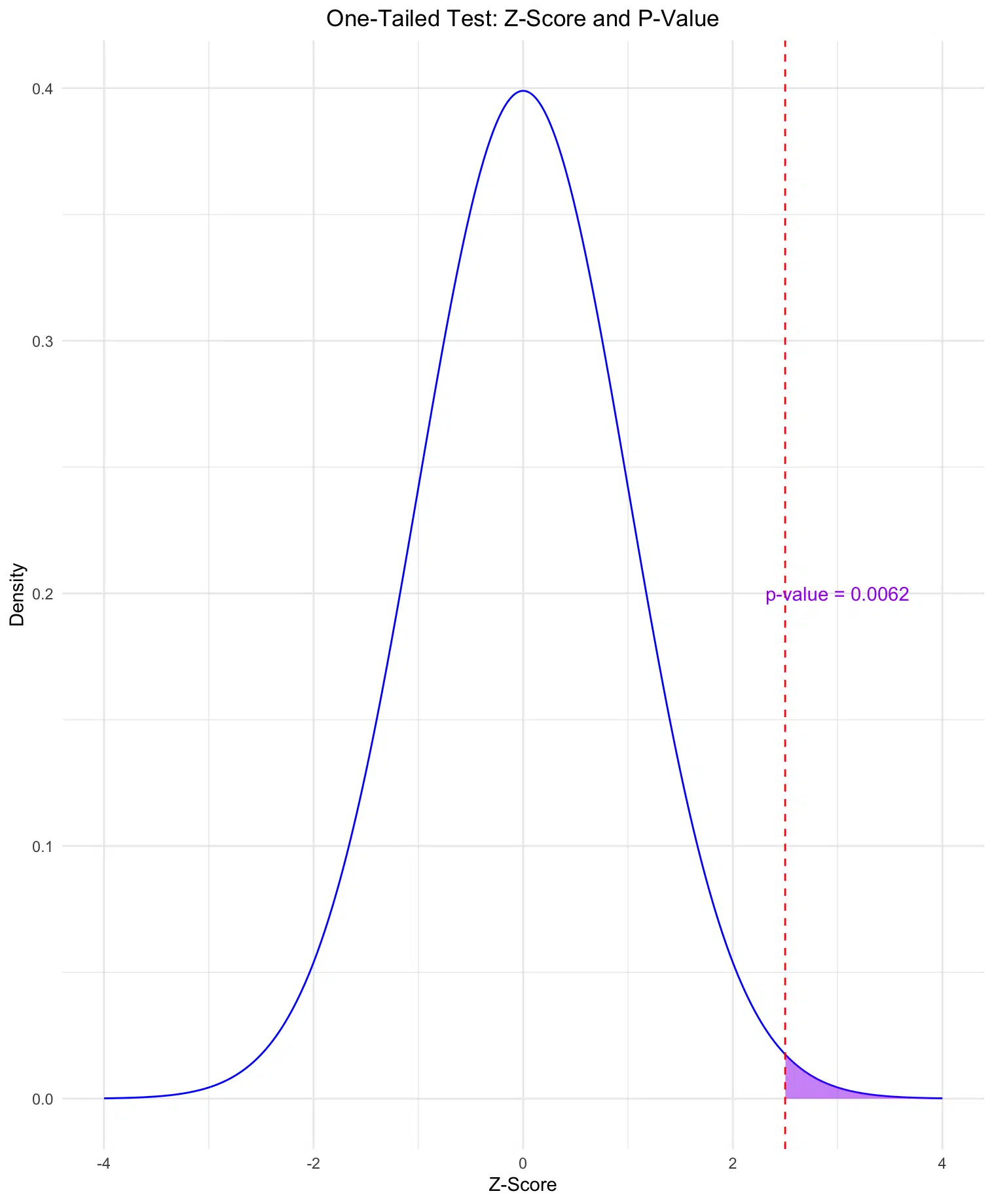
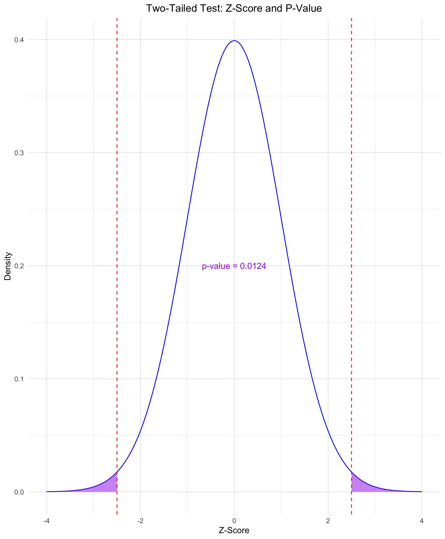
Visualizing the Z-score on a standard normal distribution allows us to see the areas representing the p-values for both one-tailed and two-tailed tests. Below, we’ll create two plots: one showing the area for a one-tailed test and another for a two-tailed test, with the calculated p-values displayed on each plot.

Example: Plotting the One-Tailed P-Value

In a one-tailed test, the p-value is the probability of observing a value as extreme as the Z-score or more in one direction (e.g., greater than the Z-score).

# Load ggplot2 for plotting
library(ggplot2)

# Z-score value
z_score <- 2.5

# Calculate one-tailed p-value
p_value_one_tailed <- pnorm(z_score, lower.tail = FALSE)

# Generate data for the standard normal distribution
x <- seq(-4, 4, length = 1000)
y <- dnorm(x)

# One-Tailed Plot
ggplot(data.frame(x, y), aes(x, y)) +
  geom_line(color = "blue") +

  # Shade for one-tailed p-value
  geom_area(data = subset(data.frame(x, y), x >= z_score), aes(x, y), fill = "purple", alpha = 0.5) +

  labs(title = "One-Tailed Test: Z-Score and P-Value",
       x = "Z-Score",
       y = "Density") +

  # Add vertical line for the Z-score
  geom_vline(xintercept = z_score, color = "red", linetype = "dashed") +

  # Add annotation for the p-value
  annotate("text", x = z_score + 0.5, y = 0.2, label = paste("p-value =", round(p_value_one_tailed, 4)), color = "purple") +

  # Center the title
  theme_minimal() +
  theme(plot.title = element_text(hjust = 0.5))

One-Tailed Test: The first plot shows the area in the right tail (purple) representing the p-value for a one-tailed test, with the calculated p-value displayed.

Example: Plotting the Two-Tailed P-Value

In a two-tailed test, the p-value is the probability of observing a value as extreme as the Z-score in either direction (both greater than and less than the mean). This accounts for extreme values on both sides of the distribution.

# Calculate two-tailed p-value
p_value_two_tailed <- 2 * pnorm(abs(z_score), lower.tail = FALSE)

# Two-Tailed Plot
ggplot(data.frame(x, y), aes(x, y)) +
  geom_line(color = "blue") +

  # Shade for two-tailed p-value
  geom_area(data = subset(data.frame(x, y), x >= z_score), aes(x, y), fill = "purple", alpha = 0.5) +
  geom_area(data = subset(data.frame(x, y), x <= -z_score), aes(x, y), fill = "purple", alpha = 0.5) +

  labs(title = "Two-Tailed Test: Z-Score and P-Value",
       x = "Z-Score",
       y = "Density") +

  # Add vertical lines for the Z-score on both sides
  geom_vline(xintercept = c(z_score, -z_score), color = "red", linetype = "dashed") +

  # Center annotation for the two-tailed p-value
  annotate("text", x = 0, y = 0.2, label = paste("p-value =", round(p_value_two_tailed, 4)), color = "purple") +

  # Center the title
  theme_minimal() +
  theme(plot.title = element_text(hjust = 0.5))

Two-Tailed Test: The second plot shows the areas in both tails (left and right) representing the p-value for a two-tailed test. The calculated p-value is displayed on the plot, providing a visual representation of the probability in both directions.

These visualizations help to interpret p-values by illustrating the areas under the curve that correspond to the observed Z-score, giving a clearer understanding of one-tailed versus two-tailed tests.

Conclusion

Calculating the p-value from a Z-score in R is straightforward with the pnorm function, enabling quick statistical tests and hypothesis evaluations. By understanding one-sided and two-sided p-values, we can interpret our test results accurately and determine if observed values significantly differ from expectations under the null hypothesis.

With this method, you can calculate p-values for Z-scores in any hypothesis testing scenario, allowing for clear, evidence-based decision-making in your statistical analyses.

Try the Z-Score to P-Value Calculator

To quickly calculate the p-value from a Z-score for your own data, check out our Z-Score to P-Value Calculator on the Research Scientist Pod.

Happy fun and happy researching!