How to Place Two Plots Side by Side using ggplot2 and cowplot in R

The easiest way to place two plots side by side using ggplot2 is to install gridExtra and then use the grid.arrange() function. For example,

install.packages("gridExtra")

grid.arrange(plot1, plot2, ncol=2)

This tutorial will go through how to place two plots side by side using ggplot2 and cowplot in R with code examples.

---

Example Using gridExtra

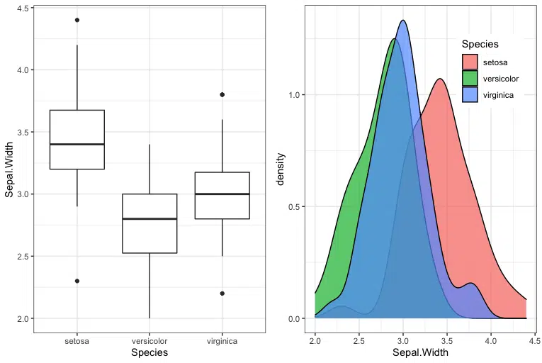
Let’s look at an example of plotting a boxplot and a density plot side-by-side. We will use the iris dataset and plot the Sepal width against Species for the boxplot and the Sepal width for the density plot.

Install ggplot2 and gridExtra

First, we need to install ggplot2 and gridExtra. The gridExtra library provides several user-level functions to work with “grid” graphics. gridExtra is commonly used to arrange multiple grid-based plots on a page and draw tables.

install.packages("gridExtra")
install.packages("ggplot2")

Plot Data Using ggplot2

Once we have installed the two packages, we can load them and define the plots. As iris is a built-in R dataset, we do not need to prepare it and can pass it as the first argument to the ggplot() constructor. In the aesthetics mappings, we will specify Species as the x-variable and Sepal.Width as the y-variable.

library(gridExtra)
library(ggplot2)

iris1 <- ggplot(iris, aes(x=Species, y = Sepal.Width)) + 
geom_boxplot() + theme_bw()

iris2 <- ggplot(iris, aes(x=Sepal.Width, fill=Species)) +
geom_density(alpha=0.7) + theme_bw() + 
theme(legend.position = c(0.8, 0.8))

We define the theme of the plots as dark-on-light using theme_bw(). We can change the transparency of the density plot using the alpha parameter.

We can assemble the two plots side-by-side using the grid.arrange() function from the gridExtra package as follows:

grid.arrange(iris1, iris2, ncol=2)

Save plot using ggsave

The grid.arrange() function returns a ggplot2 object which we can save to PDF using ggsave() as follows:

plt <- grid.arrange(iris1, iris2, ncol=2)
ggsave("side_by_side_plot.pdf", plt)

Example Using cowplot

Let’s look at how to plot the same data using cowplot. The cowplot package provides several features for creating publication-quality figures, including themes, functions to align and arrange plots, and annotation.

Install cowplot

First, we need to install cowplot.

install.packages("cowplot")

Plot Graphs Side-by-Side using cowplot

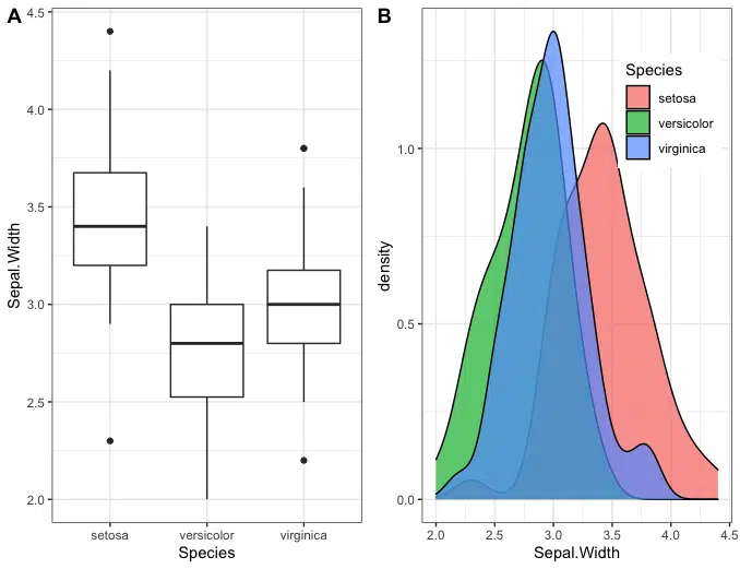
Once we have installed cowplot, we can create the ggplot2 objects and then use the function plot_grid() to arrange the plots side-by-side.

library(ggplot2)

iris1 <- ggplot(iris, aes(x=Species, y = Sepal.Width)) + 
geom_boxplot() + theme_bw()

iris2 <- ggplot(iris, aes(x=Sepal.Width, fill=Species)) +
geom_density(alpha=0.7) + theme_bw() + 
theme(legend.position = c(0.8, 0.8))

cowplot::plot_grid(iris1, iris2, labels = "AUTO")

We call the cowplot function directly without loading the package in the above code. We can call cowplot functions by prepending cowplot:: to the function.

We can also load the package and then call the plot_grid() function to achieve the same result.

library(ggplot2)
library(cowplot)
iris1 <- ggplot(iris, aes(x=Species, y = Sepal.Width)) + 
geom_boxplot() + theme_bw()

iris2 <- ggplot(iris, aes(x=Sepal.Width, fill=Species)) +
geom_density(alpha=0.7) + theme_bw() + 
theme(legend.position = c(0.8, 0.8))

plot_grid(iris1, iris2, labels = "AUTO")

Save plot using save_plot

The cowplot save_plot() function is a wrapper around ggsave() that provides added functionality to adjust the dimensions for combined plots. We can save the above figure to a PDF using the following code:

plt <- plot_grid(iris1, iris2, labels = "AUTO")
save_plot("side_by_side_cowplot.pdf", plt, ncol=2)

The parameter ncol=2 tells save_plot() that there are two plots side-by-side, then save_plot() ensures the saved image is twice as wide.

Summary

Congratulations on reading to the end of this tutorial!

For further reading on plotting in R, go to the article:

• How to Order Bars in ggplot2 Bar Graph with R

Go to the online courses page on R to learn more about coding in R for data science and machine learning.

Have fun and happy researching!