Pandas is an open-source library providing high-performance, easy-to-use data structures, and data analysis tools for Python. It is one of the fundamental tools for data scientists and can be thought of like Python’s Excel. With Pandas, you can work with many different data formats, including CSV, JSON, Excel files, SQL, and HTML. Data analysis with Pandas is intuitive. As it is Python native, the necessary code to write is very readable, making it an ideal tool for beginners in programming and data science. Pandas is built on the NumPy package, and its primary data structure is a DataFrame – a table of rows and columns. Pandas is often used in tandem with SciPy for statistical analysis, Matplotlib for visualization, and Scikit-learn for machine learning.
If you have no experience with the Python programming language before starting this tutorial, you should build up a foundation where you are confident about the basics. You can find the best Python online courses for all experience levels on the Online Courses page. It would be best if you also familiarize yourself with NumPy due to the significant overlap with Pandas.
Table of contents
About Pandas
Pandas used primarily for the cleaning, transforming, and analysis of data. Data is viewed as a table (DataFrame), which can be used to calculate statistics and answer questions about the data. For example:
- Correlation between columns.
- Average, median, and max of each column.
- The skewness of the data in a column.
- Clean data by removing missing values.
- Selecting data by condition sets.
- Visualize data using histograms, box plots, bubbles, and more.
How To Do The Tutorial
Jupyter Notebooks are a good environment for this tutorial and allow you to execute particular cells without running an entire file. You can use notebooks to work with large datasets efficiently and perform iterative transformations. You can also visualize DataFrames and plots within Notebooks. You can find the notebook with all the code in the tutorial on Github here.
How to Install Pandas
Pandas can be installed in two ways:
- PIP
- Anaconda
From your terminal you can use either of the following commands depending on your preferred package installer.
Install Pandas using PIP
pip install pandasInstall Pandas using Anaconda
conda install pandas To install Pandas from a Jupyter notebook you can use
!pip install pandasImporting Pandas
To get start using Pandas, you need to import it. Typically, in data science, we abbreviate the library to a shorthand (because of how frequently it is used). Import NumPy alongside
import pandas as pd
import numpy as np
Creating Objects From Scratch
The two primary data structures used in Pandas are the Series and the DataFrame.
Series
A Series is a one-dimensional array, treated as a column of a DataFrame. This array is capable of holding any data type. The basic method to create a Series is to call:
s = pd.Series(data, index=index)Here, data can take the form of :
- a Python dict
- an ndarray
- a scalar value
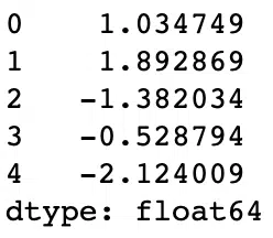
For example, using a ndarray. If no index is specified then one will be created having values [0, …., length(data) – ].
s = pd.Series(np.random.randn(5))Output:
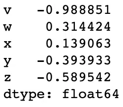
s = pd.Series(np.random.randn(5), index=['v', 'w', 'x', 'y', 'z'])Output:
Dataframe
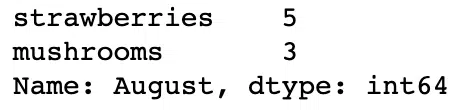
To create a DataFrame from scratch easily, you can use a dict. For example if we want to organize stock data for a green-grocers we could define the data as:
data = {
    'strawberries':[4, 5, 5, 3, 1],
    'mushrooms':[0, 0, 3, 4, 6]
}

stock = pd.DataFrame(data)
Output:
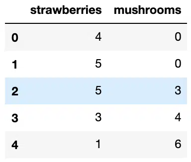
Each key of the dictionary corresponds to a column in the resulting DataFrame. The default index of the DataFrame is given on creation as explained in the Series section. We can create our own index for the DataFrame. For example we could use the months that the stock numbers were recorded:
stock = pd.DataFrame(data, index=['June', 'July', 'August', 'September', 'October'])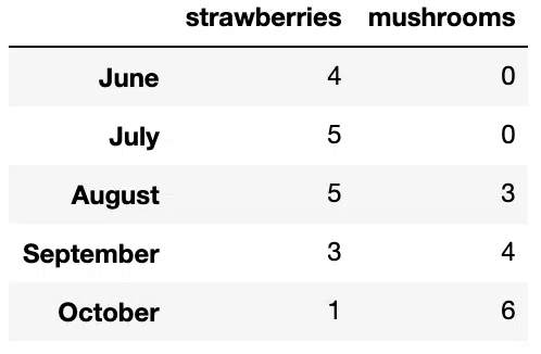
We can select a particular month to find number of crates of strawberries and mushrooms using the .loc method.
stock.loc['August']Output:
Understanding Data
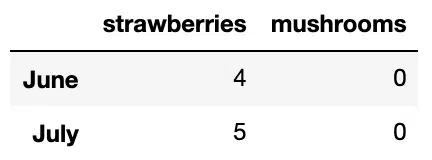
When you are looking at a new dataset, you want to see what the first few rows look like. We can use .head(n) where n is the number of rows you want to observe. If you do not include a number, the default number of rows printed is five:
#Show the top 2 rows of your dataset
stock.head(2)
Output:
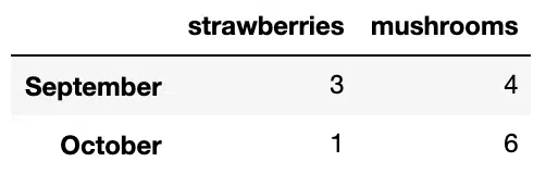
To see the bottom n rows, we can use tail(n), with n being the number of rows up from the last one in the DataFrame:
#Show bottom 2 rows of dataset
stock.tail(2)
Output:
To get a complete DataFrame description prior to any manipulation we can use info(). This method provides the essential details about the dataset including the number of rows and columns, the number of non-null values, the type of data in each column and the total memory usage of the DataFrame. This command is particularly useful for quick inspection of data to ensure any future analysis you do fits to the structure and the data types of the DataFrame.
#Get information about your data
stock.info()
Output:

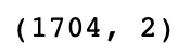
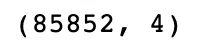
In addition to info(), we can use shape to find the number of rows and columns of the DataFrame.. The shape of a DataFrame is useful to track as we clean and transform our data. For example if we filter out rows with null values, we can found out how many rows were removed.
#Get shape of dataset as a tuple of (rows, columns)
stock.shape
Output:

Accessing Data
Here is a link for the dataset to download for the tutorial.
CSV
Comma-Separated Value files (csv) are probably the most common data source for creating DataFrames. To load in the data we can use the read_csv(filename) method.
#Read from CSV
df = pd.read_csv('data/netflix_titles.csv')
df
Output:

We can assign an index to the DataFrame from the read_csv using index_col.
#Read from CSV assign an index
df = pd.read_csv('data/netflix_titles.csv', index_col='title')
Output:

JSON
A JSON is analogous to a stored Python dict and can be read using read_json:
#Read from JSON
df = pd.read_json('data/netflix_titles.json')
Output:
Pandas automatically creates a DataFrame from the structure of the JSON but may need to use the orient keyword to make sure it gets it right. The information on the orient argument can be found in the read_json docs.
Excel
To read an XLS file, we can use read_excel(filename)
#Read from XLS
df = pd.read_excel('data/netflix_titles.xls')
Output:
Databases
When handling an SQL database, we have to establish a connection and then pass a query to Pandas. In this example we use SQLite, which can be installed from the terminal with this command:
pip install pysqlite3The following lines of code demonstrate creating a database from a CSV file:
#Create database from DataFrame

df = pd.read_csv('data/netflix_titles.csv', index_col='title')
import sqlite3
conn = sqlite3.connect('data/netflix_titles.db')
df.to_sql('films', con=conn)
We can make a connection to the database file and read out the columns using execute:
#Loading DataFrame from Database
conn = sqlite3.connect('data/netflix_titles.db')
conn.execute("SELECT * from films limit 2").fetchall()
Output:

And in turn we perform the SELECT query using read_sql_query to read from the films table and create a DataFrame:
df = pd.read_sql_query(select * from films;" conn)
df['type']
Output:

df.head()Output:

We can convert our DataFrame to a file type of our choice using the following commands:
df.to_csv('netflix_titles.csv')
df.to_excel('netflix_titles.xls')
df.to_json('netflix_titles.json')
df.to_sql('output', con)
Grouping
Pandas GroupBy is a powerful functionality that allows us to adopt a split-apply-combine approach to a dataset to answer questions we may have. GroupBy splits the data based on column(s)/condition(s) into groups and then applies a transformation to all the groups and combines them. In the example below, we want to only include films from the top 21 countries, where the number of film titles ranks countries. We use group by country and number of titles and sort in descending order. We then apply a lambda function to exclude films from countries outside of the top 21. We verify the number of unique countries using the nunique() functionality.
#Using groupby and lambda function
top_countries = df.groupby('country')['title'].count().sort_values().index
df['country'] = df.country.apply(lambda x: 'Others' if (x not in top_countries[-20:]) else x)
df['country'].nunique()
Output:

Pivoting
A Pivot table is a table that summarises the data of a more extensive table. This summary could include sums, averages, and other statistics. We can use Pandas’ pivot_table to summarise data. In the example below, we are using the Gapminder dataset, which describes the population, life expectancy, and Gross Domestic Product (GDP) per Capita of the world’s countries. We can read a CSV file from a URL using read_csv.
#Get Gapminder Dataset
url = 'http://bit.ly/2cLzoxH'
data = pd.read_csv(url)
data.head(3)
Output:

We select two columns from the DataFrame, continent and gdpPercap.
# Select two columns from dataframe
df = data[['continent','gdpPercap']]
df.shape
Output:
We want to explore the variability in GDP per capita across continents. To do that, we use pivot_table and specify which variable we would like to use for columns (continent) and which variable we would like to summarise (gdpPercap). The third argument to pivot_table is the summary method, if left unchanged the default is a mean aggregation (agg_func).
# Example of pivot_table
pd.pivot_table(df, values='gdpPercap',
              columns='continent')
Output:

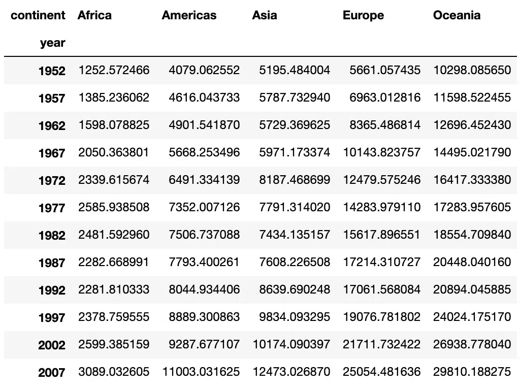
We can use more than two columns, below we explore the variability of GDP per capita across multiple years. We specify that we want the pivot table to be indexed by year:
# Pivot table with three columns from dataframe
df1 = data[['continent', 'year', 'gdpPercap']]
pd.pivot_table(df1, values='gdpPercap',
              index=['year'],
              columns='continent')
Output:
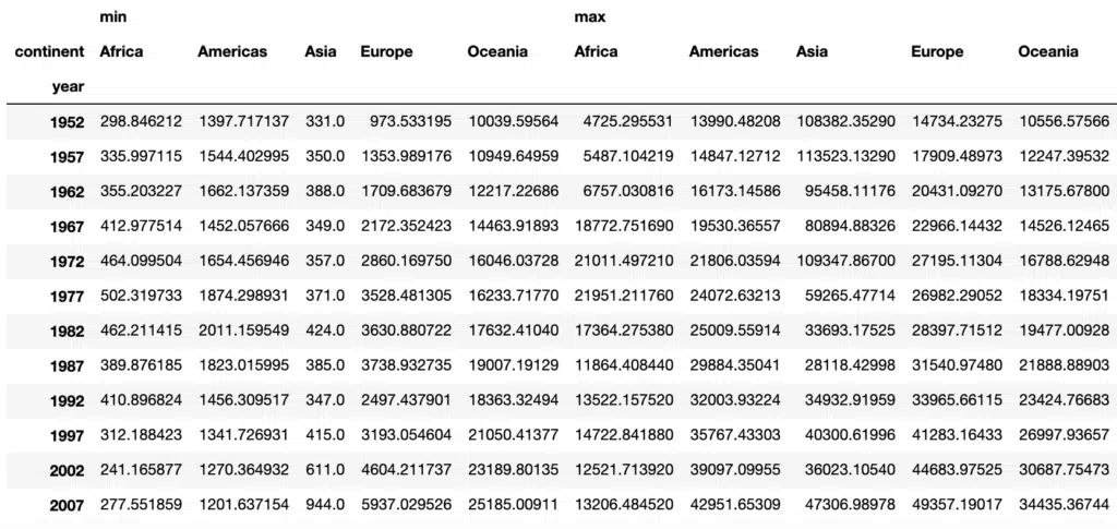
Pivot_table uses the mean function for aggregation by default, we can change the aggregating function for example taking the minimum by setting aggfunc=’min’ . This will give use the minimum gdpPerCap instead of the mean for each year and continent.
# Pivot_table with Different Aggregating Functions
pd.pivot_table(df1, values='gdpPercap',
              index=['year'],
              columns='continent',
              aggfunc='min')
Output:

We can specify more than one aggregating function. For example if we want to get the minimum and maximum values of gdpPercap for each yeah and continent, we can specify the functions as a list to the aggfunc argument:
# Pivot table with Min and Max Aggregate Functions
pd.pivot_table(df1, values='gdpPercap',
              index=['year'],
              columns='continent',
              aggfunc=[min,max])
Output:
Joining
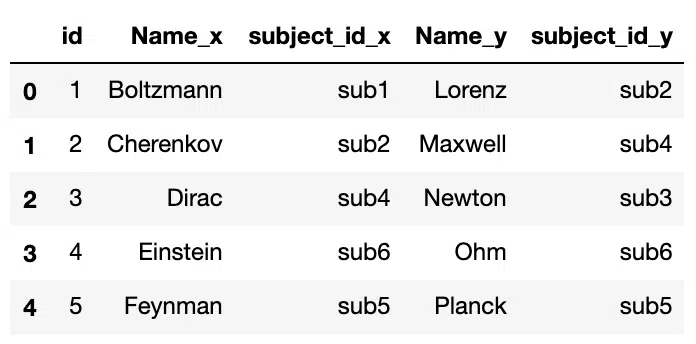
Merging or joining in Pandas is an essential skill for data science. It is the process of bringing two datasets into one and aligning the rows from each based on their shared attributes or columns. Merge and Join are used interchangeably in Pandas and other languages such as R and SQL. In the examples below we use the merge function. The definitions of Joins (merges) are shown in the figure below.

Taking two DataFrames with famous Physicists and the subject ID their work falls under for a hypothetical degree course we have:
df1 = pd.DataFrame({'id':[1,2,3,4,5],
                   'Name':['Boltzmann','Cherenkov','Dirac', 'Einstein','Feynman'],
                   'subject_id':['sub1', 'sub2', 'sub4', 'sub6', 'sub5']})

df2 = pd.DataFrame({'id':[1,2,3,4,5],
                   'Name':['Lorenz','Maxwell', 'Newton', 'Ohm', 'Planck'],
                   'subject_id':['sub2', 'sub4', 'sub3', 'sub6', 'sub5']})
Merge Two Dataframes on a Key
To merge we need to specify the two DataFrames to combine (df1 and df2) and the common column (or key) to merge on using the on argument.
#Merge two Dataframes on a Key
pd.merge(df1, df2, on='id')
Output:
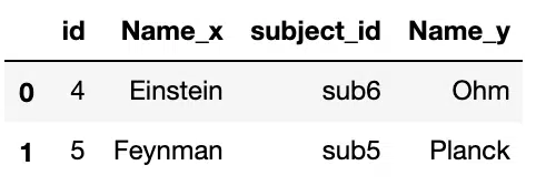
Merge Dataframes on Multiple Keys
We can merge on multiple keys by passing a list to the on argument:
#Merge two Dataframes on Multiple Keys
pd.merge(df1, df2, on=['id','subject_id'])
Output:
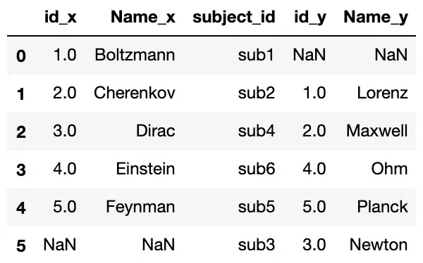
Left Join
The Left Join produces a complete set of records from the left DataFrame (df1), with the matching records (where available) in the right DataFrame (df2). We can perform a left join by passing left to the how argument of merge.
#Left Join Using "How" Argument
pd.merge(df1, df2, on='subject_id', how='left')
Output:
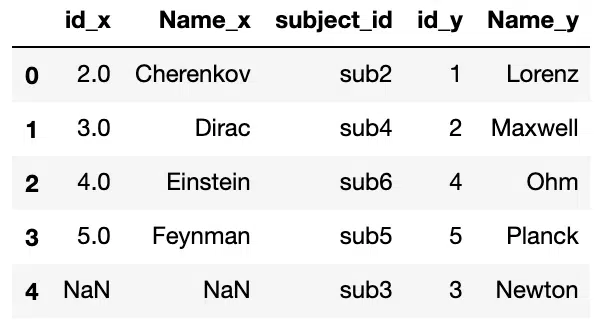
Right Join
The Right Join produces a complete set of records from the right DataFrame (df2), with the matching records (where available) in the left DataFrame (df1). We can perform a right join by passing right to the how argument of merge.
#Right Join using "How" Argument
pd.merge(df1, df2, on='subject_id', how='right')
Output:
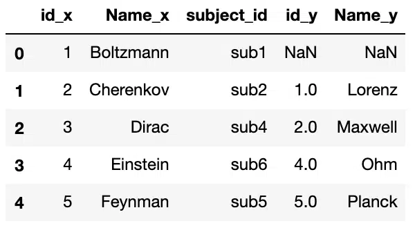
Outer Join
The Full Outer Join combines the results of both the left and right outer joins. The joined DataFrame will contain all records from both the DataFrames and fill in NaNs for missing matches on either side. We can perform a full outer join by passing outer to the how argument of merge..
#Outer Join using "How" Argument
pd.merge(df1, df2, on='subject_id', how='outer')
Output:
Notice that the resulting DataFrame has all entries from both of the tables with NaN values for missing matches on either sides. Suffixes have also been appended to the column names to show which column name came from which DataFrame. The default suffixes are x and y, butt these can be modifieed by specifying the suffixes argument in merge.
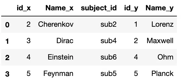
Inner Join
The Inner Join produces a set of records that match in both the left and right DataFrame. To perform an inner join, we need to pass inner to the how argument of merge.
#Inner Join using "How" Argument
pd.merge(df1, df2, on='subject_id', how='inner')
Output:
Drop
It is common to encounter missing or null values, which are placeholders for non-existent values. The equivalent in Python is None and numpy.nan for NumPy. We can check the total number of nulls in each column of our dataset using the isnull():
#Finding null values in columns
df.isnull()
Output:
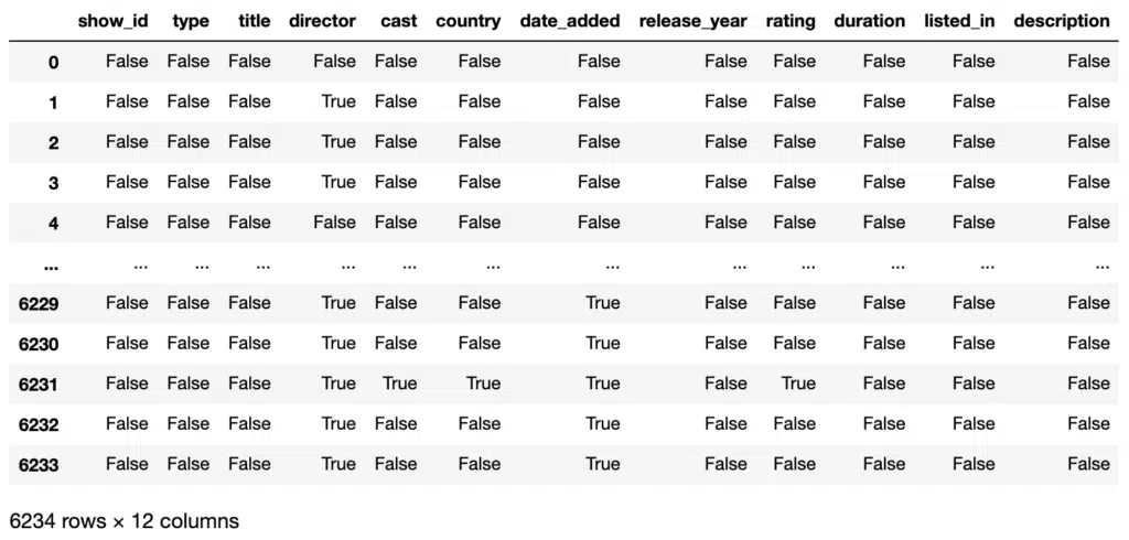
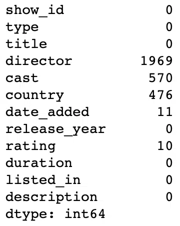
isnull returns a DataFrame with the null status of each cell. We can extract the total number of nulls in each columns using the sum aggregate function:
#Summing null values for each column
df.isnull().sum()
Output:
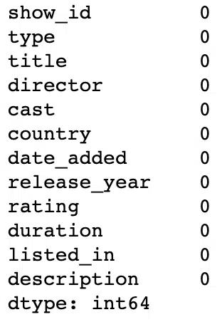
As a data scientist, the decision to drop null values is not necessarily trivial. We typically require intimate understanding of the data before dropping values universally. In general, it is recommended to remove null data if there is a relative small amount of missing data. To remove nulls, we use the dropna() functionality, which will delete any row with at least a single null value and return a new DataFrame without altering the original.
#Drop null values from columns
df = df.dropna()
df.isnull().sum()
Output:
Drop Duplicates
We can demonstrate the ability to remove duplicates by appending the DataFrame with itself.
#Adding duplicates
df = pd.read_csv('netflix_titles.csv')
df = df.append(df)
df.shape
Output:

We can drop the duplicates using the drop_duplicates() functionality.
#Dropping duplicates
df = df.drop_duplicates()
df.shape
Output:

The DataFrame shape shows that our rows have halved and is now the original shape. Instead of creating a copy of the DataFrame, we can use the inplace argument and set it to true to modify the DataFrame object in place.
#Using inplace argument for drop_duplicates
df.drop_duplicates(inplace=True)
df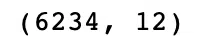
The other key argument for drop_duplicates() is keep, which specifies which duplicates to retain:
- first: (default) Drop duplicates except for the first occurrence.
- last: Drop duplicates except for the last occurrence.
- False: Drop all duplicates
Defaulting to first means the second row is dropped while retaining the first. If we set keep to False, this treats all rows as duplicates and so all of them are dropped:
#Dropping All Duplicate Rows
df = df.append(df)
df.drop_duplicates(inplace=True, keep=False)
df.shape
Output:
Manipulating Dataframes
Renaming
Datasets are rarely clean and often have column titles with odd characters, typos, spaces or mixes of lower and upper case words. Fortunately, Pandas has functionalities available to help clean up data. First we can list the columns of our Netflix DataFrame:
#Print columns
df.columns
Output:

We want to replace release_year with Release Year as a test. We set the inplace argument, so that we do not create a duplicate:
#Rename columns
df.rename(columns={'release_year': 'Release Year'}, inplace=True)
df.columns
Output:

If we want to ensure each column title is lower case, we can use a list comprehension:
#Lowercase Columns
df.columns = [col.lower() for col in df]
df.columns
Output:

Extracting By Column
We can extract columns from DataFrames by specifying the column title in square brackets:
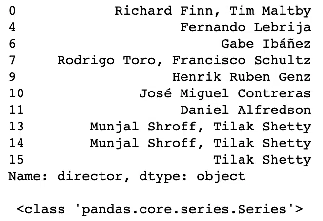
#Extract Column to Series
df = df.dropna()
directors = df['director']
print(directors.head(10), '\n\n', type(directors))
Output:
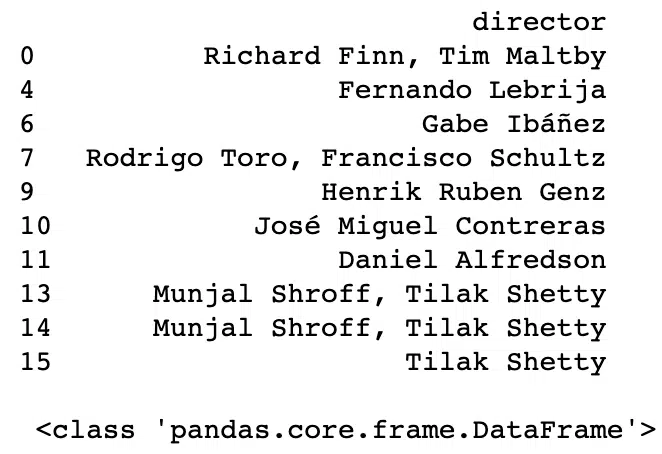
This column extraction will return a Series. To extract a column as a DataFrame, we need a list of column names:
#Extract Column to DataFrame
directors = df[['director']]
print(directors.head(10), '\n\n', type(directors))
Output:
Extracting By Row
To extract by rows, we have two options:
- .loc: locates rows by name.
- .iloc: locates rows by numerical index
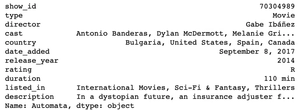
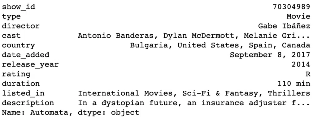
As our DataFrame is indexed by movie title, we can use .loc on the title of the movie of interest:
#Extract Row Using loc
df.loc['Automata']
Output:
And we can get the equivalent film using .iloc by passing the numerical index of Automata.
#Extract Row Using iloc
df.iloc[2]
Output:
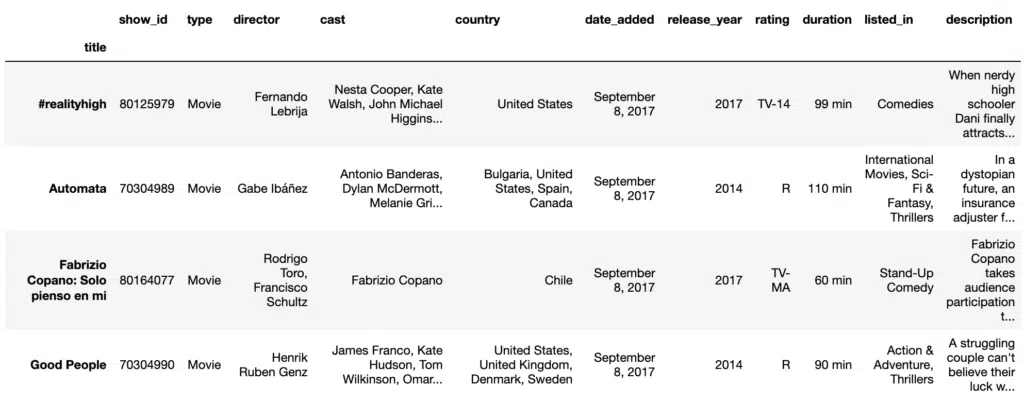
These two methods are similar to list slicing, which means we can select multiple rows with both:
#Slicing DataFrame using loc
film_collection = df.loc['#realityhigh':'Good People']
film_collection
Output:

To get the equivalent result with b we need to use y+1 in iloc[x:y] because .iloc follows the same rules as slicing with lists, the row at the end of the index is not included. So instead of 4, we use 5. If you specify an index value out of the dimensions of the DataFrame when using iloc, you will raise the error “IndexError: single positional indexer is out-of-bounds“.
#Slicing DataFrame using iloc
film_collection = df.iloc[1:5]
film_collection
Output:
Conditional Selection
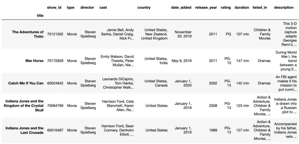
Conditional selections are very useful for when we want to extract specific items of data that fit a criteria. For example, if we are fans of Steven Spielberg’s films we may want to find all of the films available in the DataFrame. We can do this by applying a Boolean condition to the DataFrame:
#Conditional Selection
spielberg = df[df['director'] == 'Steven Spielberg']
spielberg.head(5)
Output:
Here is an example of using multiple functionalities to convert the duration column to numerical (to_numeric) and select films that are longer than three hours. We can use replace to remove the “min” appendage for the values in the duration column.
#Conditional Selection Using Numerical Values
df = pd.read_csv('data/netflix_titles.csv', index_col='title')
films = df[df['type'] == 'Movie']
films['duration']= films['duration'].str.replace(' min', '')
films['duration'] = pd.to_numeric(films['duration'], errors ='coerce')
films[films['duration'] >= 180].head(5)
Output:

Query
Query is a tool for generating subsets from a DataFrame. We have seen the loc and iloc methods to retrieve subsets based on row and column labels or by integer index of the rows and columns. These tools can be a bit bulky as they use the Pandas bracket notation. Query can be used with other Pandas methods in a streamlined fashion, making data manipulation smooth and straightforward. The parameters of query are the expression and inplace. Expression is a logical expression presented as a Python string that describes which rows to return in the output. Inplace enables us to specify if we want to directly modify the DataFrame or create a copy. We can use query to select films longer than three hours similar to the conditional selection:
films.query('duration > 180')Output:

FillNa
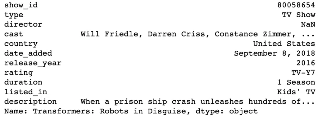
Previously we showed that dropping null values can be too severe for rows and columns with valuable data. We can perform imputation, which involves replacing null values with another value. Typically for numerical columns, null values would be replaced by the mean or median of that column. In the example below, we fill the missing value of Directors for a particular TV Series.
#Find N/A value
df = pd.read_csv("data/netflix_titles.csv", index_col='title')
df = df.loc['Transformers: Robots in Disguise']
Output:
We use loc to find the film and replace the NaN value with the list of directors.
#Fill N/A
df = df.loc['Transformers: Robots in Disguise'].fillna("David Hartman, Vinton Heuck, Scooter Tidwell, Frank Marino,Todd Waterman")
df
Output:
Note that we also had 476 null values for the country column. We can replace that with the most common (mode) country:
country = df['country']
most_common_country = country.mode()
print(most_common_country[0])
Output:
Now we have the most common country we can perform the imputation using fillna:
country.fillna(most_common_country[0], inplace=True)
df.isnull().sum()
Output:

We can see that the null values in the country column have been filled. We can increase the granularity of the imputation by selecting on specific genres or directors, which would increase the accuracy of the imputed values.
Replace
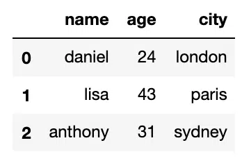
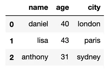
Replace Value Anywhere
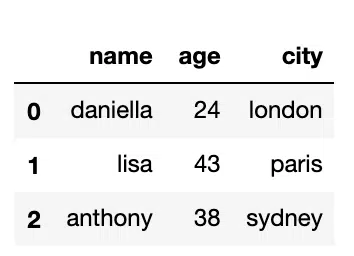
We can find and replace all instances of a value throughout the DataFrame by using the replace() functionality. Here we have a simple example of three people with ages and locations. We want to replace one age, which was mistakenly recorded:
#Replace Value Anywhere
import pandas as pd
df = pd.DataFrame({
    'name': ['daniel', 'lisa', 'anthony'],
    'age':[24, 43, 31],
    'city':['london', 'paris', 'sydney']
})
Output:
df.replace([24], 40)Output:
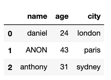
Replace With Dict
If we have multiple specific values to replace we can specify them in a Python dict:
#Replace with Dict
df.replace({
    31:38,
    'daniel':'daniella'
})
Output:
Replace With Regex
We can use regular expressions to wildcard match with values in the DataFrame and replace with a single term, in this Lisa wants to be replaced with ANON:
#Replace with Regex
df.replace('li.+','ANON', regex=True)
Output:
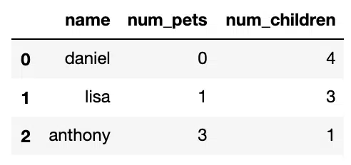
Replace in Single Column
We can reduce the scope of the replace function by specifying the column name and then the replacement to be performed:
#Replace in single column
df = pd.DataFrame({
    'name':['daniel', 'lisa', 'anthony'],
    'num_pets':[0, 1, 3],
    'num_children': [4, 3, 0]
})

#Replace 0 with 1 in column 'num_children' only
df.replace({'num_children':{0:1}})
Output:
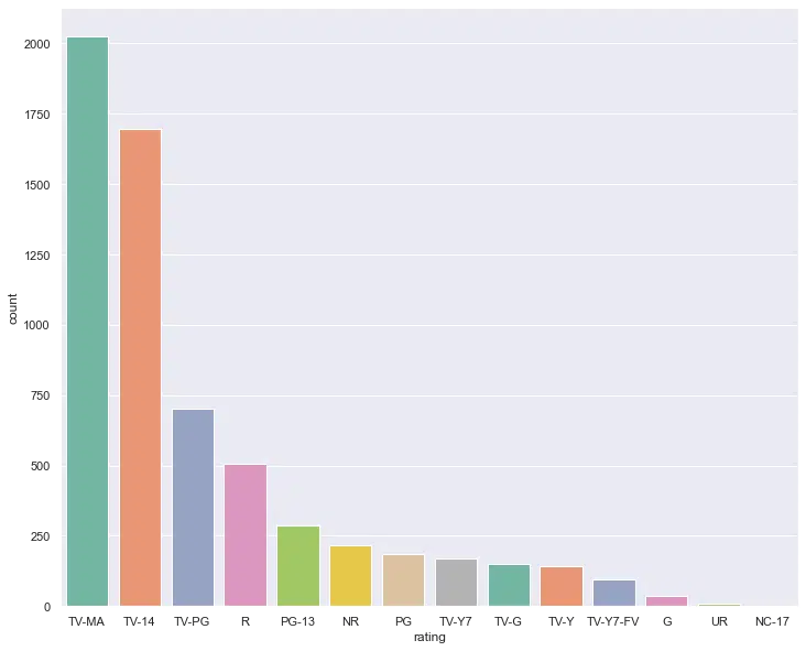
Visualization
Pandas integrates well with visualization libraries including Matplotlib, Seaborn, and plotly. We can plot directly from DataFrames and Series. The example below shows a histogram for the counts of film ratings across the entire Netflix dataset. Before using Matplotlib and Seaborn, you will have to install it from your terminal using:
pip install matplotlib
pip install seaborn
import matplotlib.pyplot as plt
import seaborn as sns
plt.figure(figsize=(12,10))
sns.set(style='darkgrid')
ax = sns.countplot(x='rating', data=df, palette="Set2", order = df['rating'].value_counts().index[0:15])Output:
We can use plotly for further visualization. In this example, we want to analyze the IMDB ratings for the films available on Netflix. We can install plotly from our terminal using:
pip install plotly We can then get the ratings for all the films in the IMDB dataset:
import plotly.express as px

imdb_ratings = pd.read_csv('data/IMDb ratings.csv', usecols=['weighted_average_vote'])
imdb_titles = pd.read_csv('data/IMDb movies.csv', usecols=['title', 'year', 'genre'])
netflix_overall = pd.read_csv('data/netflix_titles.csv')
netflix_overall.dropna()
ratings = pd.DataFrame({'Title':imdb_titles.title,
                    'Release Year':imdb_titles.year,
                    'Rating': imdb_ratings.weighted_average_vote,
                    'Genre':imdb_titles.genre})

ratings.drop_duplicates(subset=['Title','Release Year','Rating'], inplace=True)
ratings.shape
Output:
We then want to do an inner join with the Netflix dataset to find which IMDb rated films exist on Netflix.
ratings.dropna()
merged = ratings.merge(netflix_overall, left_on='Title', right_on='title',
                      how='inner')
merged = merged.sort_values(by='Rating', ascending=False)
Using plotly, we can visualize the countries with the highest rated content and the highest rated film.
#Visualiize highest rated content across countries
top_rated = merged[0:10]
fig = px.sunburst(top_rated,
                 path=['title', 'country'],
                 values='Rating',
                 color='Rating')
fig.show()
Output:

Summary
Using Pandas for data wrangling, analysis, and visualization is an essential skill for data scientists. As a data scientist, a lot of time and effort is spent cleaning and extracting data features. Pandas helps make this process as streamlined and interpretable as possible. To continue building your knowledge beyond the beginner level, you can go through the official Pandas extended tutorials. Practise is the best way to understand how Pandas works and grow confident using it, so you should also look through Kaggle projects with fun datasets and start building your own projects.
Thank you for going through this tutorial to the end. As a beginner, I hope you have gained some knowledge about Pandas and now know where it fits in the data science utility belt. For online courses that use Pandas, please visit the Online Courses Page, in particular, the Applied Data Science with Python Specialization course under the Data Science page. Stay tuned for more tutorials on essential tools for data science!

Suf is a senior advisor in data science with deep expertise in Natural Language Processing, Complex Networks, and Anomaly Detection. Formerly a postdoctoral research fellow, he applied advanced physics techniques to tackle real-world, data-heavy industry challenges. Before that, he was a particle physicist at the ATLAS Experiment of the Large Hadron Collider. Now, he’s focused on bringing more fun and curiosity to the world of science and research online.