How to Calculate Mean Squared Error (MSE) in R with a Real-Life Example

Mean Squared Error (MSE) is a popular metric for evaluating the accuracy of models in machine learning and statistics. It measures the average squared difference between the observed values and those predicted by a model, giving insight into the model’s performance. In this post, we’ll cover how to calculate MSE in R using an easy-to-understand example, and we’ll include a plot to visually compare the actual and predicted values.

What is Mean Squared Error?

MSE is defined as:

\[ \text{MSE} = \frac{1}{n} \sum_{i=1}^{n} (y_i – \hat{y}_i)^2 \]

where:

• \( n \) is the number of observations,
• \( y_i \) is the actual value of the \( i \)-th observation,
• \( \hat{y}_i \) is the predicted value of the \( i \)-th observation.

Smaller MSE values indicate that predictions are close to the actual values, while larger values show a greater average error.

Real-Life Example: Predicting House Prices

Let’s say you’re a real estate agent trying to predict house prices based on certain features (e.g., square footage, location, number of bedrooms). You’ve built a model that estimates house prices, and now you want to see how accurate your predictions are using MSE.

Here’s some hypothetical data showing the actual prices of recently sold houses and the prices your model predicted:

# Actual house prices (in thousands of dollars)
actual <- c(300, 150, 200, 400, 500)

# Predicted house prices by the model
predicted <- c(320, 180, 190, 410, 450)

In this example:

• actual represents the true selling prices,
• predicted represents the prices estimated by your model.

Step 1: Manually Calculating MSE in R

To calculate the MSE, we’ll follow these steps:

1. Calculate the difference between each actual and predicted value.
2. Square each difference.
3. Find the average of these squared differences.

Let’s go through these steps in R:

# Step 1: Calculate the differences
differences <- actual - predicted

# Step 2: Square the differences
squared_differences <- differences^2

# Step 3: Calculate the mean of the squared differences
mse <- mean(squared_differences)
mse

Running this code will give the MSE:

[1] 700

This tells us that, on average, the squared error of our predictions is 700 (in thousands of dollars squared). In other words, the model’s predictions are off by a considerable amount, on average.

Step 2: Visualizing Observed vs. Predicted Values

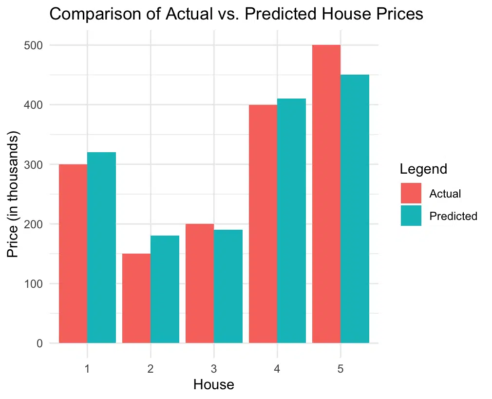
To better understand where the predictions deviate from the actual values, let’s plot them side by side. Here’s how to create a bar chart showing the actual vs. predicted house prices for each house:

# Load the necessary packages
library(ggplot2)
library(reshape2)

# Create a data frame for plotting
data <- data.frame(
  House = factor(1:5),
  Actual = actual,
  Predicted = predicted
)

# Reshape data for easy plotting
data_long <- melt(data, id.vars = "House")

# Plot observed vs. predicted prices
ggplot(data_long, aes(x = House, y = value, fill = variable)) +
  geom_bar(stat = "identity", position = "dodge") +
  labs(title = "Comparison of Actual vs. Predicted House Prices",
       x = "House",
       y = "Price (in thousands)",
       fill = "Legend") +
  theme_minimal()

This plot provides a side-by-side view of actual and predicted prices for each house. Each bar group represents a house, and the Actual and Predicted bars are displayed next to each other, making it easy to see where the predictions were accurate and where they were off.

Step 3: Creating an MSE Function for Reusability

Calculating MSE manually can be time-consuming, so let’s create a simple function to calculate MSE whenever needed.

# Define a function to calculate MSE
calculate_mse <- function(actual, predicted) {
  mean((actual - predicted)^2)
}

# Use the function
mse <- calculate_mse(actual, predicted)
mse

This function makes it easy to compute MSE with any actual and predicted values. Just call calculate_mse(actual, predicted), and it will return the MSE.

Step 4: Using the Metrics Package for MSE

Alternatively, R’s Metrics package provides a mse() function to calculate MSE directly.

1. First, install the package if you haven’t already:

install.packages("Metrics")

2. Load the package and use the mse() function:

library(Metrics)

mse <- mse(actual, predicted)
mse

This package’s mse() function provides a straightforward way to calculate MSE for larger datasets.

Interpreting the MSE Value and Plot

The MSE value tells us the average squared error of our model’s predictions. In our house price example, the MSE of 700 means that our model’s price predictions are, on average, off by $26,457 (since the square root of 700,000 is approximately $26,457). The plot also visually highlights which predictions were close to the actual values and where larger discrepancies occurred, helping us gain a more intuitive understanding of the model’s accuracy.

Conclusion

Calculating MSE in R is simple and valuable for evaluating model performance. By using a real-life example like house price prediction and visualizing the actual vs. predicted values, we can better understand where the model is performing well and where it may need improvement. This approach to assessing model accuracy is essential for building reliable models in data-driven projects.

Try the MSE Calculator

If you’d like to calculate MSE quickly for your own data, check out our Mean Squared Error Calculator on Research Data Pod.

Have fun and happy researching!