How to Calculate Root Mean Squared Error (RMSE) in R with a Real-Life Example

Root Mean Squared Error (RMSE) is a commonly used metric for evaluating the accuracy of predictions in machine learning and statistics. It provides a measure of the average magnitude of errors between observed and predicted values. In this post, we’ll explain RMSE, demonstrate how to calculate it in R with an easy-to-understand example, and visualize the results.

What is Root Mean Squared Error?

RMSE is the square root of the Mean Squared Error (MSE) and is defined as:

\[ \text{RMSE} = \sqrt{\frac{1}{n} \sum_{i=1}^{n} (y_i – \hat{y}_i)^2} \]

where:

• \( n \) is the number of observations,
• \( y_i \) is the actual value of the \( i \)-th observation,
• \( \hat{y}_i \) is the predicted value of the \( i \)-th observation.

RMSE provides a measure of the prediction errors’ magnitude, making it a valuable metric for regression models.

Real-Life Example: Predicting Temperature

Let’s say you’re a meteorologist trying to predict daily high temperatures based on historical data. You’ve developed a model to estimate these temperatures, and now you want to assess how accurate your predictions are using RMSE.

Here’s some hypothetical data showing the actual daily high temperatures and the temperatures predicted by your model:

# Actual temperatures (in degrees Celsius)
actual <- c(22, 25, 28, 20, 23, 26, 27)

# Predicted temperatures by the model
predicted <- c(21, 24, 29, 19, 22, 25, 28)

In this example:

• actual represents the true temperatures,
• predicted represents the temperatures estimated by your model.

Step 1: Manually Calculating RMSE in R

To calculate the RMSE, we’ll follow these steps:

1. Calculate the difference between each actual and predicted value.
2. Square each difference.
3. Find the mean of these squared differences (this is the Mean Squared Error).
4. Take the square root of the Mean Squared Error to obtain the RMSE.

Here’s how to calculate RMSE in R:

# Step 1: Calculate the differences
differences <- actual - predicted

# Step 2: Square the differences
squared_differences <- differences^2

# Step 3: Calculate the mean of the squared differences (MSE)
mse <- mean(squared_differences)

# Step 4: Take the square root of MSE to get RMSE
rmse <- sqrt(mse)
rmse

Running this code will give the RMSE:

[1] 1.0

This tells us that, on average, the model’s temperature predictions have an error magnitude of about 1 degree Celsius.

Step 2: Visualizing Observed vs. Predicted Values

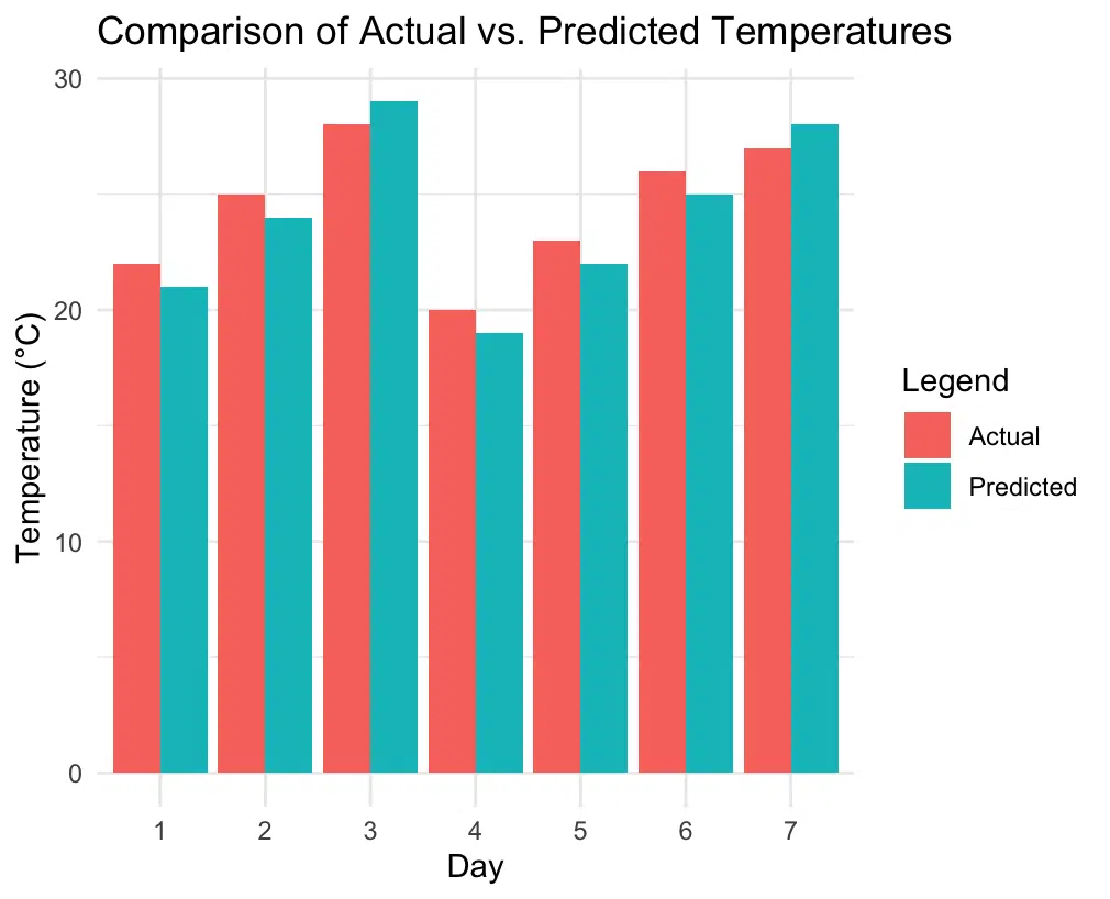
To get a better understanding of the prediction accuracy, let’s create a plot comparing the actual and predicted temperatures for each day:

# Load the necessary packages
library(ggplot2)
library(reshape2)

# Create a data frame for plotting
data <- data.frame(
  Day = factor(1:7),
  Actual = actual,
  Predicted = predicted
)

# Reshape data for easy plotting
data_long <- melt(data, id.vars = "Day")

# Plot observed vs. predicted temperatures
ggplot(data_long, aes(x = Day, y = value, fill = variable)) +
  geom_bar(stat = "identity", position = "dodge") +
  labs(title = "Comparison of Actual vs. Predicted Temperatures",
       x = "Day",
       y = "Temperature (°C)",
       fill = "Legend") +
  theme_minimal()

This plot provides a visual comparison of actual and predicted temperatures for each day, allowing us to see where the model predictions were close or further from the actual values.

Step 3: Creating an RMSE Function for Reusability

Calculating RMSE manually can be time-consuming, so let’s create a simple function to calculate RMSE whenever needed.

# Define a function to calculate RMSE
calculate_rmse <- function(actual, predicted) {
  sqrt(mean((actual - predicted)^2))
}

# Use the function
rmse <- calculate_rmse(actual, predicted)
rmse

Now, you can compute RMSE with any actual and predicted values using calculate_rmse(actual, predicted).

Step 4: Using the Metrics Package for RMSE

Alternatively, R’s Metrics package provides an rmse() function to calculate RMSE directly.

1. First, install the package if you haven’t already:

install.packages("Metrics")

2. Load the package and use the rmse() function:

library(Metrics)

rmse <- rmse(actual, predicted)
rmse

This package’s rmse() function provides a straightforward way to calculate RMSE for larger datasets.

Interpreting the RMSE Value and Plot

The RMSE value indicates the average magnitude of prediction errors. In our temperature example, an RMSE of 1.0 means that our model’s temperature predictions are, on average, off by about 1 degree Celsius. The plot helps illustrate where predictions were accurate and where there were larger deviations.

Conclusion

Calculating RMSE in R is an essential skill for any statistician or data scientist, offering a clear, interpretable measure of prediction accuracy. In our temperature prediction example, RMSE highlights both the strengths and limitations of the model, providing a quantifiable view of performance. By assessing RMSE, we gain valuable insight into how well our model generalizes to real data, guiding us in refining models for improved accuracy and reliability. RMSE remains a foundational tool for robust model evaluation in predictive analytics.

Try the RMSE Calculator

If you’d like to calculate RMSE quickly for your own data, check out our Root Mean Squared Error Calculator on the Research Scientist Pod.

Have fun and happy researching!