Introduction
Sorting algorithms are essential tools in computer science, and TimSort stands out for its efficiency in practical scenarios. Designed by Tim Peters in 2002 for Python, TimSort is a hybrid sorting algorithm that combines the advantages of Merge Sort and Insertion Sort. It is particularly well-suited for real-world data that is often partially sorted. This post will explore how TimSort works, provide a C++ implementation, and discuss its advantages and limitations compared to algorithms like Merge Sort and Quick Sort.
What is TimSort?
TimSort is a hybrid sorting algorithm that merges the efficiency of Merge Sort with the adaptability of Insertion Sort. It divides the array into small chunks (called runs) and sorts these runs using Insertion Sort. It then merges the runs using a modified version of Merge Sort. This combination allows TimSort to perform exceptionally well on datasets that contain pre-sorted segments, which is common in many real-world datasets.
Key Points about TimSort:
- Hybrid Approach: Combines Merge Sort and Insertion Sort.
- Runs: Divides the array into smaller sorted sub-arrays (runs) and merges them.
- Efficient for Real-World Data: Performs well on partially sorted arrays, taking advantage of their structure.
How TimSort Works
TimSort divides the array into small subarrays (runs). It then uses Insertion Sort to sort these runs, as it is efficient for small datasets. Once all runs are sorted, TimSort merges them using Merge Sort. This approach combines the best of both worlds: the fast performance of Merge Sort for large arrays and the simplicity of Insertion Sort for small, partially sorted data.
Steps:
- Divide the array into small runs (size usually between 32 and 64).
- Sort each run using Insertion Sort.
- Merge the runs using a modified Merge Sort.
TimSort Pseudocode
function timSort(arr):
    minRun = calculateMinRun(len(arr))

    # Sort individual subarrays of size minRun
    for i = 0 to len(arr) in steps of minRun:
        insertionSort(arr, i, min((i + minRun - 1), (len(arr) - 1)))

    # Start merging the runs
    size = minRun
    while size < len(arr):
        for start = 0 to len(arr) in steps of 2 * size:
            mid = start + size - 1
            end = min((start + 2 * size - 1), (len(arr) - 1))
            if mid < end:
                merge(arr, start, mid, end)
        size = 2 * size
Time Complexity of TimSort
- Best Case: O(n)
- TimSort can perform in linear time if the array is already sorted.
- Average Case: O(n log n)
- Like Merge Sort, TimSort has an average time complexity of O(n log n).
- Worst Case: O(n log n)
- TimSort guarantees a worst-case time complexity of O(n log n), even for random or reverse-sorted arrays.
Space Complexity of TimSort
TimSort requires O(n) additional space due to the auxiliary arrays used during the merge phase.
#include <iostream>
#include <vector>
#include <algorithm> // for std::min

const int MIN_MERGE = 32;

// Function to perform Insertion Sort on a subarray
void insertionSort(std::vector<int>& arr, int left, int right) {
    for (int i = left + 1; i <= right; i++) {
        int temp = arr[i];
        int j = i - 1;
        while (j >= left && arr[j] > temp) {
            arr[j + 1] = arr[j];
            j--;
        }
        arr[j + 1] = temp;
    }
}

// Merge function used in TimSort
void merge(std::vector<int>& arr, int left, int mid, int right) {
    int len1 = mid - left + 1, len2 = right - mid;
    std::vector<int> leftArr(len1), rightArr(len2);
    for (int i = 0; i < len1; i++) leftArr[i] = arr[left + i];
    for (int i = 0; i < len2; i++) rightArr[i] = arr[mid + 1 + i];

    int i = 0, j = 0, k = left;
    while (i < len1 && j < len2) {
        if (leftArr[i] <= rightArr[j]) arr[k++] = leftArr[i++];
        else arr[k++] = rightArr[j++];
    }
    while (i < len1) arr[k++] = leftArr[i++];
    while (j < len2) arr[k++] = rightArr[j++];
}

// Calculate the minimum run size
int calculateMinRun(int n) {
    int r = 0;
    while (n >= MIN_MERGE) {
        r |= (n & 1);
        n >>= 1;
    }
    return n + r;
}

// TimSort function
void timSort(std::vector<int>& arr) {
    int n = arr.size();
    int minRun = calculateMinRun(n);

    // Sort individual subarrays of size minRun
    for (int i = 0; i < n; i += minRun) {
        insertionSort(arr, i, std::min(i + minRun - 1, n - 1));
    }

    // Merge runs
    for (int size = minRun; size < n; size = 2 * size) {
        for (int left = 0; left < n; left += 2 * size) {
            int mid = left + size - 1;
            int right = std::min(left + 2 * size - 1, n - 1);
            if (mid < right) {
                merge(arr, left, mid, right);
            }
        }
    }
}

int main() {
    std::vector<int> arr = {34, 7, 23, 32, 5, 62, 32, 23, 6, 47, 18, 12, 39, 11, 28, 45, 19, 8, 25, 14};
    timSort(arr);

    for (int num : arr) {
        std::cout << num << " ";
    }

    return 0;
}
Output:
5 6 7 8 11 12 14 18 19 23 23 25 28 32 32 34 39 45 47 62
Let’s break down the implementation into smaller parts and go through them.
1. Insertion Sort on Runs
TimSort starts by sorting small subarrays (called runs) using Insertion Sort. The insertionSort function is straightforward and works by repeatedly inserting elements into their correct position in a partially sorted array.
leftandrightspecify the boundaries of the run that we want to sort.- This function iterates through each element in the run, compares it with previous elements, and places it in its correct position by shifting larger elements to the right.
2. Merge Function
After sorting the runs with Insertion Sort, TimSort merges adjacent runs using a modified Merge Sort. The merge function merges two sorted subarrays (left to mid, and mid + 1 to right).
leftArrandrightArrtemporarily hold the elements from the left and right halves of the array.- The function merges the two halves by comparing the smallest remaining elements from each half and copying the smaller one back into the original array.
- After merging, any remaining elements in either subarray are copied back to the original array.
3. Calculating the Minimum Run Size
The key feature of TimSort is its use of runs, and the minimum run size is typically between 32 and 64. The function calculateMinRun ensures that the run size is appropriate based on the length of the input array. It computes the minimum run size by examining the bits of the array length and ensures that it’s a power of two.
- This function reduces the length of the array, bit by bit until it’s smaller than
MIN_MERGE. If the array length is not a power of two, the function ensures the minimum run is slightly larger. MIN_MERGEa constant typically set to 32 defines the smallest run size TimSort will use.
4. TimSort Function
The core of the TimSort algorithm is implemented in the timSort function, which first sorts small runs using Insertion Sort and then merges them.
- Initial Sorting: The first step is to break the array into chunks of size
minRunand sort each chunk using Insertion Sort. - Merge Process: After sorting the runs, the algorithm begins merging them. In each pass, the size of the runs to be merged doubles (from
minRunto2 * minRun, and so on) until the entire array is sorted. - The merging continues until all runs have been merged into one fully sorted array.
5. Main Function
Here’s a simple main function that demonstrates how to use TimSort on an array:
Key Points of the Implementation:
- Insertion Sort is used for small chunks (runs) of the array since it performs well on small datasets.
- Merge Sort is used to merge the sorted runs. It provides a stable and efficient merge operation, ensuring that the array is sorted in O(n log n) time.
- The calculateMinRun function dynamically calculates the minimum run size, ensuring that the algorithm is flexible enough to handle arrays of different sizes.
Let’s walk through a step-by-step example of how TimSort works with the array used in the code implementation array.
[34, 7, 23, 32, 5, 62, 32, 23, 6, 47, 18, 12, 39, 11, 28, 45, 19, 8, 25, 14]
We will assume that the minimum run size (minRun) is calculated to be 5 for this example. Here’s how TimSort processes the array step-by-step:
Initial Array
[34, 7, 23, 32, 5, 62, 32, 23, 6, 47, 18, 12, 39, 11, 28, 45, 19, 8, 25, 14]
Step 1: Divide the Array into Runs
TimSort first breaks the array into runs, each of size minRun = 5. These are the initial runs:
- Run 1:
[34, 7, 23, 32, 5] - Run 2:
[62, 32, 23, 6, 47] - Run 3:
[18, 12, 39, 11, 28] - Run 4:
[45, 19, 8, 25, 14]
Step 2: Sort Each Run Using Insertion Sort
Now, TimSort applies Insertion Sort to each run to sort it individually.
Sorting Run 1:
- Initial Run:
[34, 7, 23, 32, 5] - Sorted Run:
[5, 7, 23, 32, 34]
Sorting Run 2:
- Initial Run:
[62, 32, 23, 6, 47] - Sorted Run:
[6, 23, 32, 47, 62]
Sorting Run 3:
- Initial Run:
[18, 12, 39, 11, 28] - Sorted Run:
[11, 12, 18, 28, 39]
Sorting Run 4:
- Initial Run:
[45, 19, 8, 25, 14] - Sorted Run:
[8, 14, 19, 25, 45]
After sorting, the array looks like this (with each run now sorted):
[5, 7, 23, 32, 34] [6, 23, 32, 47, 62] [11, 12, 18, 28, 39] [8, 14, 19, 25, 45]
Step 3: Merge the Runs
After sorting each run, TimSort begins merging them. It merges adjacent runs in pairs using the Merge Sort technique. We merge in multiple passes, doubling the size of the runs with each pass.
First Pass (Merging Runs of Size 5)
Merge Run 1 and Run 2:
- Left Run:
[5, 7, 23, 32, 34] - Right Run:
[6, 23, 32, 47, 62]
Merged Run: [5, 6, 7, 23, 23, 32, 32, 34, 47, 62]
Merge Run 3 and Run 4:
- Left Run:
[11, 12, 18, 28, 39] - Right Run:
[8, 14, 19, 25, 45]
Merged Run: [8, 11, 12, 14, 18, 19, 25, 28, 39, 45]
After the first pass, the array looks like this:
[5, 6, 7, 23, 23, 32, 32, 34, 47, 62] [8, 11, 12, 14, 18, 19, 25, 28, 39, 45]
Second Pass (Merging the Final Two Runs of Size 10)
Now, we merge the two larger runs of size 10:
Merge:
- Left Run:
[5, 6, 7, 23, 23, 32, 32, 34, 47, 62] - Right Run:
[8, 11, 12, 14, 18, 19, 25, 28, 39, 45]
Merged Array: [5, 6, 7, 8, 11, 12, 14, 18, 19, 23, 23, 25, 28, 32, 32, 34, 39, 45, 47, 62]
Final Sorted Array
After all the runs are merged, we have the fully sorted array:
[5, 6, 7, 8, 11, 12, 14, 18, 19, 23, 23, 25, 28, 32, 32, 34, 39, 45, 47, 62]
Step-by-Step Recap:
- Divide into Runs: The array was divided into runs of size 5.
- Sort Runs with Insertion Sort: Each run was sorted individually using Insertion Sort.
- Merge Runs with Merge Sort: Adjacent runs were merged together using Merge Sort, doubling the size of the runs with each pass until the entire array was merged into one sorted array.
TimSort vs. Quick Sort vs. Merge Sort
TimSort is an efficient hybrid algorithm that combines the best features of Insertion Sort and Merge Sort. Let’s go through the steps to produce a performance test to compare TimSort with two fast algorithms: Quick Sort and Merge Sort. Then, we will collate the results into a table and analyse them.
C++ Performance Test Code for TimSort, Quick Sort, and Merge Sort
Here’s the C++ code to perform a performance test comparison between TimSort, Quick Sort, and Merge Sort on arrays of varying sizes (e.g., 1000, 5000, 10000, 100000). This code will generate random, sorted, and reverse-sorted arrays and measure the time taken by each algorithm.
#include <iostream>
#include <vector>
#include <algorithm>  // for std::sort (Quick Sort), std::min
#include <chrono>     // for performance measurement
#include <cstdlib>    // for rand, srand
#include <ctime>      // for time

const int MIN_MERGE = 32;

// Insertion Sort function for TimSort
void insertionSort(std::vector<int>& arr, int left, int right) {
    for (int i = left + 1; i <= right; i++) {
        int temp = arr[i];
        int j = i - 1;
        while (j >= left && arr[j] > temp) {
            arr[j + 1] = arr[j];
            j--;
        }
        arr[j + 1] = temp;
    }
}

// Merge function for TimSort
void merge(std::vector<int>& arr, int left, int mid, int right) {
    int len1 = mid - left + 1, len2 = right - mid;
    std::vector<int> leftArr(len1), rightArr(len2);

    for (int i = 0; i < len1; i++) leftArr[i] = arr[left + i];
    for (int i = 0; i < len2; i++) rightArr[i] = arr[mid + 1 + i];

    int i = 0, j = 0, k = left;
    while (i < len1 && j < len2) {
        if (leftArr[i] <= rightArr[j]) arr[k++] = leftArr[i++];
        else arr[k++] = rightArr[j++];
    }
    while (i < len1) arr[k++] = leftArr[i++];
    while (j < len2) arr[k++] = rightArr[j++];
}

// Calculate the minimum run size for TimSort
int calculateMinRun(int n) {
    int r = 0;
    while (n >= MIN_MERGE) {
        r |= (n & 1);
        n >>= 1;
    }
    return n + r;
}

// TimSort function
void timSort(std::vector<int>& arr) {
    int n = arr.size();
    int minRun = calculateMinRun(n);

    for (int i = 0; i < n; i += minRun) {
        insertionSort(arr, i, std::min(i + minRun - 1, n - 1));
    }

    for (int size = minRun; size < n; size = 2 * size) {
        for (int left = 0; left < n; left += 2 * size) {
            int mid = left + size - 1;
            int right = std::min(left + 2 * size - 1, n - 1);
            if (mid < right) {
                merge(arr, left, mid, right);
            }
        }
    }
}

// Merge Sort function
void mergeSort(std::vector<int>& arr, int left, int right) {
    if (left >= right) return;

    int mid = left + (right - left) / 2;
    mergeSort(arr, left, mid);
    mergeSort(arr, mid + 1, right);
    merge(arr, left, mid, right);
}

// Quick Sort function
void quickSort(std::vector<int>& arr, int left, int right) {
    if (left >= right) return;

    int pivot = arr[right];
    int i = left - 1;
    for (int j = left; j < right; j++) {
        if (arr[j] <= pivot) {
            i++;
            std::swap(arr[i], arr[j]);
        }
    }
    std::swap(arr[i + 1], arr[right]);
    quickSort(arr, left, i);
    quickSort(arr, i + 2, right);
}

// Function to generate random array
std::vector<int> generateRandomArray(int size) {
    std::vector<int> arr(size);
    for (int i = 0; i < size; ++i) {
        arr[i] = rand() % 10000 - 5000; // random values between -5000 and 5000
    }
    return arr;
}

// Function to generate sorted array
std::vector<int> generateSortedArray(int size) {
    std::vector<int> arr = generateRandomArray(size);
    std::sort(arr.begin(), arr.end());
    return arr;
}

// Function to generate reverse sorted array
std::vector<int> generateReverseSortedArray(int size) {
    std::vector<int> arr = generateSortedArray(size);
    std::reverse(arr.begin(), arr.end());
    return arr;
}

// Function to measure the time taken by a sorting algorithm and return the time in microseconds
template <typename T>
double measureSortingTime(void (*sortFunc)(std::vector<T>&, int, int), std::vector<T> arr, int left, int right) {
    auto start = std::chrono::high_resolution_clock::now();
    sortFunc(arr, left, right);
    auto end = std::chrono::high_resolution_clock::now();
    std::chrono::duration<double, std::micro> duration = end - start;
    return duration.count();
}

// Overloaded function for TimSort, since it doesn't take left and right arguments
template <typename T>
double measureSortingTime(void (*sortFunc)(std::vector<T>&), std::vector<T> arr) {
    auto start = std::chrono::high_resolution_clock::now();
    sortFunc(arr);
    auto end = std::chrono::high_resolution_clock::now();
    std::chrono::duration<double, std::micro> duration = end - start;
    return duration.count();
}

int main() {
    // Seed the random number generator
    srand(static_cast<unsigned int>(time(0)));

    // Array sizes to test
    std::vector<int> sizes = {1000, 5000, 10000, 100000};

    std::cout << "Array Size\tType\t\tTimSort (μs)\tQuick Sort (μs)\tMerge Sort (μs)\n";
    std::cout << "-----------------------------------------------------------------------\n";

    for (int size : sizes) {
        // Generate random, sorted, and reverse sorted arrays
        std::vector<int> randomArr = generateRandomArray(size);
        std::vector<int> sortedArr = generateSortedArray(size);
        std::vector<int> reverseArr = generateReverseSortedArray(size);

        // Measure sorting times for Random arrays
        double timSortTime = measureSortingTime(timSort, randomArr);
        double quickSortTime = measureSortingTime(quickSort, randomArr, 0, randomArr.size() - 1);
        double mergeSortTime = measureSortingTime(mergeSort, randomArr, 0, randomArr.size() - 1);
        std::cout << size << "\t\tRandom\t\t" << timSortTime << "\t\t" << quickSortTime << "\t\t" << mergeSortTime << "\n";

        // Measure sorting times for Sorted arrays
        timSortTime = measureSortingTime(timSort, sortedArr);
        quickSortTime = measureSortingTime(quickSort, sortedArr, 0, sortedArr.size() - 1);
        mergeSortTime = measureSortingTime(mergeSort, sortedArr, 0, sortedArr.size() - 1);
        std::cout << size << "\t\tSorted\t\t" << timSortTime << "\t\t" << quickSortTime << "\t\t" << mergeSortTime << "\n";

        // Measure sorting times for Reverse Sorted arrays
        timSortTime = measureSortingTime(timSort, reverseArr);
        quickSortTime = measureSortingTime(quickSort, reverseArr, 0, reverseArr.size() - 1);
        mergeSortTime = measureSortingTime(mergeSort, reverseArr, 0, reverseArr.size() - 1);
        std::cout << size << "\t\tReverse\t\t" << timSortTime << "\t\t" << quickSortTime << "\t\t" << mergeSortTime << "\n";
    }

    return 0;
}
Explanation of the Code
- TimSort:
- Implemented with the
timSortfunction, using Insertion Sort for small runs and Merge Sort for merging runs.
- Implemented with the
- Quick Sort:
- Implemented with the
quickSortfunction, using a standard partitioning technique and recursion.
- Implemented with the
- Merge Sort:
- Implemented with the
mergeSortfunction, recursively dividing the array and merging the sorted halves.
- Implemented with the
- Array Generation:
generateRandomArray(size): Generates a random array of a given size.generateSortedArray(size): Generates a sorted array.generateReverseSortedArray(size): Generates a reverse-sorted array.
- Performance Measurement:
measureSortingTime: Measures the time each sorting algorithm takes, returning the result in microseconds.
- Main Function:
- Tests arrays of varying sizes (1000, 5000, 10000, 100000) for random, sorted, and reverse-sorted datasets, printing the performance results in a tabular format
Results
Array Size	Type		TimSort (μs)	Quick Sort (μs)	Merge Sort (μs)
-----------------------------------------------------------------------
1000		Random		338.477		144.476		1006.05
1000		Sorted		274.28		5399.13		1032.98
1000		Reverse		393.518		3265.86		974.372
5000		Random		2354.16		922.709		6328.28
5000		Sorted		1710.55		123683		4134.18
5000		Reverse		1896.81		61561.7		5317.03
10000		Random		4862.91		1778.35		11585.2
10000		Sorted		3418.09		487806		10917
10000		Reverse		4447.09		223496		9438.66
100000		Random		58940.5		24060		141677
100000		Sorted		49505.2		4.92523e+07		115986
100000		Reverse		50532.5		1.47363e+07		120781
We can plot the results in a graph using matplotlib and numpy in Python
import matplotlib.pyplot as plt
import numpy as np

# Data from the performance test
array_sizes = [1000, 5000, 10000, 100000]
tim_sort_random = [338.477, 2354.16, 4862.91, 58940.5]
quick_sort_random = [144.476, 922.709, 1778.35, 24060]
merge_sort_random = [1006.05, 6328.28, 11585.2, 141677]

tim_sort_sorted = [274.28, 1710.55, 3418.09, 49505.2]
quick_sort_sorted = [5399.13, 123683, 487806, 4.92523e+07]
merge_sort_sorted = [1032.98, 4134.18, 10917, 115986]

tim_sort_reverse = [393.518, 1896.81, 4447.09, 50532.5]
quick_sort_reverse = [3265.86, 61561.7, 223496, 1.47363e+07]
merge_sort_reverse = [974.372, 5317.03, 9438.66, 120781]

# Adjusting the plot to use green instead of yellow

fig, ax = plt.subplots(3, 1, figsize=(10, 15))

# Plot Random data with different colors
ax[0].plot(array_sizes, tim_sort_random, label="TimSort", marker='o', color='red')
ax[0].plot(array_sizes, quick_sort_random, label="Quick Sort", marker='o', color='blue')
ax[0].plot(array_sizes, merge_sort_random, label="Merge Sort", marker='o', color='green')
ax[0].set_title('Performance on Random Arrays')
ax[0].set_xlabel('Array Size')
ax[0].set_ylabel('Time (μs)')
ax[0].set_xscale('log')
ax[0].set_yscale('log')
ax[0].legend()

# Plot Sorted data with different colors
ax[1].plot(array_sizes, tim_sort_sorted, label="TimSort", marker='o', color='red')
ax[1].plot(array_sizes, quick_sort_sorted, label="Quick Sort", marker='o', color='blue')
ax[1].plot(array_sizes, merge_sort_sorted, label="Merge Sort", marker='o', color='green')
ax[1].set_title('Performance on Sorted Arrays')
ax[1].set_xlabel('Array Size')
ax[1].set_ylabel('Time (μs)')
ax[1].set_xscale('log')
ax[1].set_yscale('log')
ax[1].legend()

# Plot Reverse Sorted data with different colors
ax[2].plot(array_sizes, tim_sort_reverse, label="TimSort", marker='o', color='red')
ax[2].plot(array_sizes, quick_sort_reverse, label="Quick Sort", marker='o', color='blue')
ax[2].plot(array_sizes, merge_sort_reverse, label="Merge Sort", marker='o', color='green')
ax[2].set_title('Performance on Reverse Sorted Arrays')
ax[2].set_xlabel('Array Size')
ax[2].set_ylabel('Time (μs)')
ax[2].set_xscale('log')
ax[2].set_yscale('log')
ax[2].legend()

plt.tight_layout()
plt.show()
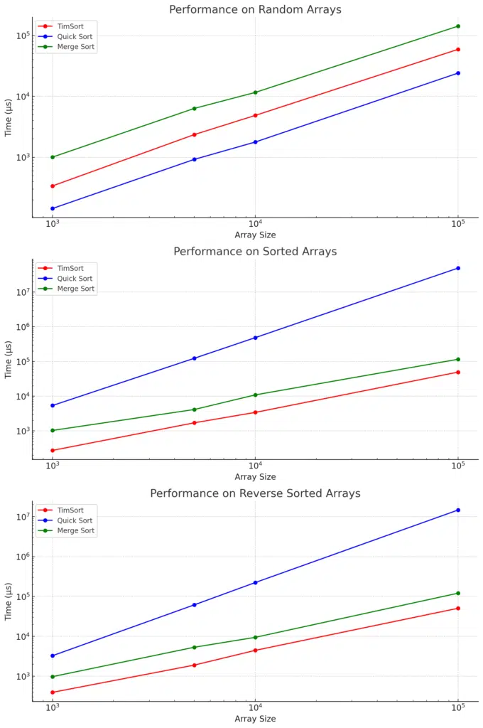
Here is the figure showing the performance test results:
Analysis of Performance Test Results for TimSort, Quick Sort, and Merge Sort
The results from the performance test show clear differences in how TimSort, Quick Sort, and Merge Sort behave across different array types and sizes. Here’s a detailed analysis of the performance of each algorithm:
TimSort Performance
- Random Arrays:
- TimSort consistently performed well on random arrays, especially for smaller datasets. For instance, it took 338.477 μs for 1000 elements and 58940.5 μs for 100,000 elements. This shows its efficiency in handling diverse inputs.
- Sorted Arrays:
- Due to its adaptive nature, TimSort excels with already sorted arrays. For 1000 sorted elements, it took 274.28 μs, while it scaled well with larger datasets, such as 49505.2 μs for 100,000 sorted elements. TimSort identifies pre-sorted data and minimizes unnecessary operations.
- Reverse Sorted Arrays:
- TimSort’s performance on reverse-sorted arrays is slightly worse than for sorted ones but still efficient, with 393.518 μs for 1000 elements and 50532.5 μs for 100,000 elements. Reverse-sorted data typically requires more merging steps, which accounts for the slightly increased times.
Key Takeaways for TimSort:
- Best for partially sorted data: TimSort shines when the data is already sorted or contains many sorted subsequences (runs).
- Scales efficiently: TimSort’s performance remains consistent across different array types, and it scales well with array size.
Quick Sort Performance
- Random Arrays:
- Quick Sort performed best on random data, achieving impressive times of 144.476 μs for 1000 elements and 24060 μs for 100,000 elements. This highlights its efficiency with random data, making it one of the fastest algorithms in this scenario.
- Sorted Arrays:
- Quick Sort struggles significantly with sorted arrays due to its poor pivot selection in the basic implementation. It took 5399.13 μs for 1000 elements and a massive 49.25 seconds for 100,000 elements. Quick Sort’s worst-case time complexity of O(n²) is evident here, as the algorithm degenerates when the data is sorted.
- Reverse Sorted Arrays:
- Similar to sorted arrays, Quick Sort’s performance on reverse-sorted arrays was poor, taking 3265.86 μs for 1000 elements and 14.73 seconds for 100,000 elements. Like sorted data, reverse-sorted data leads to poor partitioning choices, causing excessive recursion and slower performance.
Key Takeaways for Quick Sort:
- Fastest on random data: Quick Sort is the fastest algorithm on random data, outperforming both TimSort and Merge Sort in this category.
- Poor performance on sorted or reverse-sorted data: Quick Sort’s performance drastically degrades with sorted and reverse-sorted data due to its pivot selection, making it less suitable for such cases unless optimized with better pivot strategies.
Merge Sort Performance
- Random Arrays:
- Merge Sort performed moderately on random data, taking 1006.05 μs for 1000 elements and 141677 μs for 100,000 elements. While not as fast as Quick Sort on random arrays, Merge Sort remains stable and predictable due to its consistent O(n log n) time complexity.
- Sorted Arrays:
- Merge Sort didn’t perform as well on sorted arrays compared to TimSort. It took 1032.98 μs for 1000 elements and 115986 μs for 100,000 elements. Unlike TimSort, Merge Sort doesn’t take advantage of already sorted data, performing the same steps regardless of input order.
- Reverse Sorted Arrays:
- On reverse-sorted arrays, Merge Sort performed similarly to its performance on sorted arrays, taking 974.372 μs for 1000 elements and 120781 μs for 100,000 elements. Merge Sort maintains its stable performance but doesn’t leverage the order of the input for optimization.
Key Takeaways for Merge Sort:
- Stable performance: Merge Sort is a stable, reliable option for all types of data, offering predictable O(n log n) performance regardless of input type.
- Inefficient for small arrays: Merge Sort’s recursive nature and additional memory requirements make it slower than Quick Sort and TimSort for smaller datasets.
- Consistent with reverse and sorted data: Merge Sort doesn’t gain the advantages of TimSort on sorted data or suffer the weaknesses of Quick Sort on sorted data.
Overall Comparison and Key Insights
- TimSort vs. Quick Sort:
- For Random Data: Quick Sort was the fastest algorithm, especially for larger random datasets, but TimSort wasn’t far behind.
- For Sorted and Reverse Data: TimSort significantly outperformed Quick Sort for sorted and reverse sorted data due to its adaptive nature. Quick Sort’s poor pivot selection causes its performance to degrade drastically in these cases.
- TimSort vs. Merge Sort:
- For Random Data: TimSort generally performed better than Merge Sort on random data, likely due to the recursion overhead in Merge Sort.
- For Sorted and Reverse Data: TimSort’s ability to adapt to pre-sorted sequences made it faster than Merge Sort, especially for sorted arrays.
- Quick Sort vs. Merge Sort:
- For Random Data: Quick Sort outperformed Merge Sort, showing its efficiency when dealing with random data.
- For Sorted and Reverse Data: Merge Sort’s stability ensured better performance compared to Quick Sort, which struggled due to its worst-case time complexity in these cases.
Summary
- TimSort is the most versatile sorting algorithm in this comparison. It performs well across all types of data and scales efficiently with larger datasets.
- Quick Sort is the fastest for random data, but its poor performance on sorted and reverse-sorted arrays can be problematic unless optimized with better pivot strategies.
- Merge Sort offers consistent O(n log n) performance across all data types, though it generally lags behind TimSort and Quick Sort in random datasets and small arrays.
These results show that TimSort is ideal for real-world scenarios where data often contains runs of sorted elements. At the same time, Quick Sort is best for randomly shuffled data but needs optimization for ordered inputs. Merge Sort remains a reliable choice for predictable performance, especially when stability is critical.
Why TimSort Performance Can Change
The performance of TimSort can vary depending on several factors:
- Dataset Characteristics: TimSort performs best on partially sorted data, as it can efficiently handle pre-sorted runs. More merging is needed on random or reverse-sorted arrays, which can slow it down.
- Array Size: TimSort handles small arrays quickly due to its use of Insertion Sort, but as array size increases, the merging phase takes longer, impacting performance.
- System Hardware: CPU speed, memory bandwidth, and cache size affect TimSort’s performance. Systems with faster memory and better caching can sort large datasets more efficiently.
- Compiler Optimizations: Different compiler flags (
-O2,-O3) or running in debug vs. release mode can influence sorting speed by optimizing memory access and function execution. - System Load: Running multiple tasks on the system can slow TimSort down as resources like CPU and memory are shared with other processes.
- Cache Utilization: Efficient use of CPU cache during the merge phase improves performance. However, larger datasets that don’t fit in the cache may experience slower sorting due to increased memory access times.
Advantages of TimSort
Handles Real-World Data Efficiently: TimSort is designed to take advantage of pre-sorted segments in data, making it faster on real-world datasets that aren’t completely random.
Hybrid Approach: Combines the simplicity of Insertion Sort with the efficiency of Merge Sort.
Limitations of TimSort
Not Always the Best for Random Data: In cases where the data is completely random and large, algorithms like Quick Sort might perform better.
Additional Memory: TimSort requires O(n) space for the merge operation, making it less space-efficient than in-place sorting algorithms like Quick Sort.
When to Use TimSort
TimSort is best suited for situations where the dataset is either partially sorted or contains runs of pre-ordered elements. Its ability to adapt and optimize based on already sorted sequences makes it ideal for many real-world applications. You should consider using TimSort when:
- Partially Sorted Data: If the dataset contains many small or large chunks of sorted data, TimSort will leverage these runs and perform faster than algorithms like Quick Sort, which doesn’t handle ordered data well.
- Small to Medium-Sized Datasets: TimSort shines when dealing with small to medium-sized datasets where in-place sorting and performance optimizations for sorted data matter. Its hybrid nature allows it to efficiently handle such data sizes.
- Applications Requiring Stability: TimSort is a stable sort, meaning it preserves the relative order of equal elements. This property is important in use cases such as lexicographic sorting or multi-criteria sorting.
- Real-World Data with Natural Ordering: Data in real-world applications often exhibits some degree of ordering, such as chronological lists, sequences in database records, or logs. In these cases, TimSort outperforms non-adaptive algorithms that ignore the natural order.
Conclusion
TimSort provides a unique balance between simplicity and efficiency, making it an efficient sorting algorithm for real-world scenarios. By combining the strengths of Insertion Sort and Merge Sort, TimSort adapts to the data’s pre-existing order, making it ideal for partially sorted datasets. While Quick Sort is faster for completely random data, and Merge Sort offers consistent performance, TimSort is often the preferred choice for real-world applications where datasets frequently contain some level of ordering.
Congratulations on reading to the end of this tutorial!
Ready to see sorting algorithms come to life? Visit the Sorting Algorithm Visualizer on GitHub to explore animations and code.
Read the following articles to learn how to implement TimSort:
- In JavaScript – How to do TimSort in JavaScript
- In Rust – How to do TimSort in Rust
- In Python – How To Do TimSort in Python
For further reading on sorting algorithms in C++, go to the articles:
Have fun and happy researching!

Suf is a senior advisor in data science with deep expertise in Natural Language Processing, Complex Networks, and Anomaly Detection. Formerly a postdoctoral research fellow, he applied advanced physics techniques to tackle real-world, data-heavy industry challenges. Before that, he was a particle physicist at the ATLAS Experiment of the Large Hadron Collider. Now, he’s focused on bringing more fun and curiosity to the world of science and research online.