How to Calculate the P-Value of a T-Score in R with Practical Examples

In statistical analysis, the t-score helps us understand how far a sample mean is from the population mean, adjusted for sample size. Calculating the p-value from a t-score can tell us the probability of observing a value as extreme as the one observed, assuming the null hypothesis is true. This guide explores how to calculate the p-value from a t-score in R using practical examples.

Introduction to T-Scores and P-Values

The t-score is calculated as follows:

\[ T = \frac{\bar{X} – \mu}{s / \sqrt{n}} \]

where:

• \( \bar{X} \) is the sample mean,
• \( \mu \) is the population mean,
• \( s \) is the sample standard deviation, and
• \( n \) is the sample size.

Once we have the t-score, we can calculate the p-value to determine the probability of obtaining a t-score as extreme as, or more extreme than, the observed t-score under the null hypothesis.

Understanding the T-Score

A t-score helps us determine whether a sample mean is statistically different from a population mean, particularly when the sample size is small or the population standard deviation is unknown. The p-value derived from the t-score indicates the probability of observing this t-score under the null hypothesis.

Calculating the P-Value from a T-Score

To calculate the p-value from a t-score, we use the t-distribution. The p-value formula varies based on whether the test is one-tailed or two-tailed.

Formula for Calculating the P-Value

For a given t-score and degrees of freedom \( df \), the p-value is calculated as follows:

• One-Tailed Test: The p-value is given by: \[ p = P(T > |t|) = pt(|t|, df, lower.tail = FALSE) \]
• Two-Tailed Test: The p-value is given by: \[ p = 2 \times pt(|t|, df, lower.tail = FALSE) \]

In R, we can use the pt function to calculate the p-value directly. For a one-tailed test:

p_value <- pt(t_score, df, lower.tail = FALSE)

For a two-tailed test:

p_value <- 2 * pt(abs(t_score), df, lower.tail = FALSE)

Example: Calculating P-Value from a T-Score

Suppose we have a t-score of 2.5 with 15 degrees of freedom. We’ll calculate the p-value for both one-tailed and two-tailed tests:

# T-score and degrees of freedom
t_score <- 2.5
df <- 15

# One-tailed p-value
p_value_one_tailed <- pt(t_score, df, lower.tail = FALSE)

# Two-tailed p-value
p_value_two_tailed <- 2 * pt(abs(t_score), df, lower.tail = FALSE)

p_value_one_tailed
p_value_two_tailed

The output will be:

# One-tailed p-value
[1] 0.0122529

# Two-tailed p-value
[1] 0.0245058

For this example, the one-tailed p-value of 0.0122529 suggests that the probability of observing a t-score as extreme as 2.5 in one direction is about 1.2%. The two-tailed p-value of 0.0245058 indicates a 2.45% probability of observing a t-score as extreme as ±2.5 in either direction, under the null hypothesis.

Visualizing the T-Score on a T-Distribution

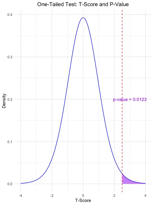
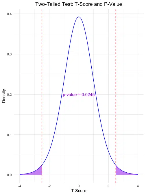
Visualizing the t-score on a t-distribution allows us to see the areas representing the p-values for one-tailed and two-tailed tests. Below, we’ll create two plots: one for a one-tailed test and another for a two-tailed test, with calculated p-values displayed on each plot.

Example: Plotting the One-Tailed P-Value

# Load ggplot2 for plotting
library(ggplot2)

# Generate data for t-distribution
x <- seq(-4, 4, length = 1000)
y <- dt(x, df)

# Calculate one-tailed p-value
p_value_one_tailed <- pt(t_score, df, lower.tail = FALSE)

# One-Tailed Plot
ggplot(data.frame(x, y), aes(x, y)) +
  geom_line(color = "blue") +
  geom_area(data = subset(data.frame(x, y), x >= t_score), aes(x, y), fill = "purple", alpha = 0.5) +
  labs(title = "One-Tailed Test: T-Score and P-Value",
       x = "T-Score",
       y = "Density") +
  geom_vline(xintercept = t_score, color = "red", linetype = "dashed") +
  annotate("text", x = t_score + 0.5, y = 0.2, label = paste("p-value =", round(p_value_one_tailed, 4)), color = "purple") +
  theme_minimal() +
  theme(plot.title = element_text(hjust = 0.5))

One-Tailed Test: The first plot shows the area in the right tail (purple) representing the p-value for a one-tailed test, with the calculated p-value displayed.

Example: Plotting the Two-Tailed P-Value

# Calculate two-tailed p-value
p_value_two_tailed <- 2 * pt(abs(t_score), df, lower.tail = FALSE)

# Two-Tailed Plot
ggplot(data.frame(x, y), aes(x, y)) +
  geom_line(color = "blue") +
  geom_area(data = subset(data.frame(x, y), x >= t_score), aes(x, y), fill = "purple", alpha = 0.5) +
  geom_area(data = subset(data.frame(x, y), x <= -t_score), aes(x, y), fill = "purple", alpha = 0.5) +
  labs(title = "Two-Tailed Test: T-Score and P-Value",
       x = "T-Score",
       y = "Density") +
  geom_vline(xintercept = c(t_score, -t_score), color = "red", linetype = "dashed") +
  annotate("text", x = 0, y = 0.2, label = paste("p-value =", round(p_value_two_tailed, 4)), color = "purple") +
  theme_minimal() +
  theme(plot.title = element_text(hjust = 0.5))

Two-Tailed Test: The second plot shows the areas in both tails (left and right) representing the p-value for a two-tailed test. The calculated p-value is displayed on the plot, providing a visual representation of the probability in both directions.

Assumptions and Limitations of Using T-Scores and P-Values

Calculating a p-value from a t-score involves certain assumptions about the data and has inherent limitations that can impact the interpretation of results. Here’s a detailed breakdown:

Assumptions

• Normality of Data: The t-test assumes that the data follows a normal distribution. This assumption is crucial, particularly when the sample size is small (n < 30). For larger samples, the Central Limit Theorem suggests that the distribution of sample means will approximate normality even if the original data is not perfectly normal.
• Independence of Observations: The observations within the data set should be independent of each other. This means that the occurrence of one data point should not influence or be influenced by another. Violations of this assumption, such as in paired or repeated measurements, can lead to incorrect conclusions if not accounted for in the testing method.
• Scale of Measurement: T-tests assume interval or ratio scales for the data, as these provide meaningful distances between values. Nominal or ordinal data cannot be appropriately analyzed using t-scores, as these scales do not convey information about the relative magnitude of differences.
• Equality of Variances (in Two-Sample T-Tests): When comparing two samples, the t-test assumes that the variances in the two groups are approximately equal. If this assumption is violated, alternative tests (e.g., Welch’s t-test) that do not assume equal variances may be more appropriate.

Limitations

• Sensitivity to Outliers: T-tests are sensitive to outliers, as extreme values can distort the mean and standard deviation, leading to misleading t-scores and p-values. If outliers are present, the results may not accurately reflect the central tendency of the data, potentially affecting the statistical significance.
• Interpretation of P-Values: A statistically significant p-value (e.g., p < 0.05) suggests that the observed effect is unlikely under the null hypothesis, but it does not indicate the effect size or practical significance. A significant p-value does not automatically imply that the result is meaningful or important, especially in large samples where even minor differences can yield small p-values.
• Does Not Account for Multiple Testing: When multiple t-tests are performed on the same dataset, the likelihood of obtaining a significant result by chance increases. Adjustments, such as the Bonferroni correction, may be necessary to control for the increased risk of Type I errors (false positives) across multiple tests.
• Dependence on Sample Size: The statistical power of the t-test is influenced by the sample size. With small samples, the t-test may lack the sensitivity to detect significant differences (increased risk of Type II errors), while in very large samples, even trivial differences may appear statistically significant due to the reduction in sampling error.
• Only Measures Difference in Means: The t-test is designed to measure differences between group means. It does not provide insights into other characteristics, such as variability or distribution shape, which may also be relevant to understanding group differences. Additional tests may be necessary to gain a more comprehensive view of the data.
• Assumes Homogeneity of Variances (in Some Tests): For two-sample t-tests assuming equal variances, any violation of this assumption can lead to inaccurate results. When variances differ significantly between groups, the use of a Welch’s t-test, which does not assume equal variances, is recommended.

By understanding these assumptions and limitations, you can better interpret t-scores and p-values and ensure your conclusions are statistically sound and contextually relevant. Proper application of the t-test and careful consideration of these factors will enhance the reliability of your results.

Conclusion

Calculating the p-value from a t-score in R is straightforward with the pt function, enabling quick hypothesis evaluations for small sample sizes. By understanding one-sided and two-sided p-values, we can accurately interpret test results to determine if observed values significantly differ from expectations under the null hypothesis.

Try the T-Score to P-Value Calculator

To quickly calculate the p-value from a t-score for your data, check out our T-Score to P-Value Calculator on the Research Scientist Pod.

Have fun and happy researching!