How To Do Insertion Sort in C++

Introduction

Insertion Sort is one of the simplest and most intuitive sorting algorithms, making it a great starting point for beginners. It works similarly to how you might sort playing cards: picking one card at a time and inserting it in the correct position among the already sorted cards.

While Insertion Sort is not efficient for large datasets due to its quadratic time complexity, it’s an excellent algorithm for small datasets or nearly sorted data.

In this post, we’ll explain how Insertion Sort works, provide pseudocode, and give you a detailed C++ implementation then go through a performance test against two other common sorting algorithms Selection and Bubble Sort.

---

What is Insertion Sort?

Insertion Sort takes one element at a time from the unsorted section and inserts it into the correct position in the sorted section. As the algorithm progresses, the sorted section grows while the unsorted section shrinks.

---

Key Points About Insertion Sort:

• Simple and easy to implement.
• Best for small or nearly sorted datasets.
• Inefficient for large datasets with a worst-case time complexity of O(n²).
• In-place sorting, so it requires only O(1) extra memory.
• Stable sorting algorithm, preserving the order of equal elements.

---

Time Complexity of Insertion Sort:

• Best Case (O(n)): The array is already sorted, and no shifting is required.
• Average Case (O(n²)): On average, about half of the elements need to be shifted.
• Worst Case (O(n²)): The array is sorted in reverse order, and every element has to be compared and shifted.

Space Complexity:

• O(1): Insertion Sort is an in-place sorting algorithm, so it doesn’t need additional memory apart from the input array.

---

Pseudocode for Insertion Sort

for i = 1 to n-1 do               // Start from the second element since the first element is already "sorted"
    key = arr[i]                  // Select the current element (key) to be inserted into the sorted portion
    j = i - 1                     // Initialize j to the index of the last element in the sorted portion
    
    // Shift elements in the sorted portion to the right if they are greater than the key
    while j >= 0 and arr[j] > key do
        arr[j + 1] = arr[j]        // Move the larger element one position to the right
        j = j - 1                  // Move to the next element on the left in the sorted portion
    end while
    
    // Insert the key into its correct position in the sorted portion
    arr[j + 1] = key               // Place the key at the position found after the shifting
end for

Explanation of Each Step:

1. Outer Loop (for i = 1 to n-1):
   • This loop starts at the second element (index 1) because the first element is considered to be in the sorted portion of the array.
   • The algorithm iterates through the entire array, picking each element one by one to insert it into the sorted portion.
2. Key Selection (key = arr[i]):
   • The current element, arr[i], is stored in the variable key. This is the element that needs to be inserted into the correct position in the sorted portion of the array.
3. Shifting Elements (while j >= 0 and arr[j] > key):
   • A while loop is used to find the correct position for the key. It checks if the current element in the sorted portion (arr[j]) is greater than the key.
   • If it is, the element is shifted one position to the right (i.e., arr[j + 1] = arr[j]), making room for the key.
   • This continues until an element smaller than or equal to the key is found, or until we reach the start of the array (j = -1).
4. Inserting the Key (arr[j + 1] = key):
   • Once the correct position is found, the key is inserted by placing it in the appropriate position (arr[j + 1]).
   • This ensures that the array remains sorted from arr[0] to arr[i].

---

C++ Implementation of Insertion Sort:

Here’s the full C++ implementation using the larger array:

#include <iostream>
using namespace std;

// Function to perform insertion sort
void insertionSort(int arr[], int n) {
    for (int i = 1; i < n; i++) {
        int key = arr[i];  // Element to be inserted
        int j = i - 1;
        
        // Move elements of arr[0..i-1], that are greater than key, one position ahead
        while (j >= 0 && arr[j] > key) {
            arr[j + 1] = arr[j];  // Shift element to the right
            j = j - 1;
        }
        arr[j + 1] = key;  // Insert the key in its correct position
    }
}

// Function to print an array
void printArray(int arr[], int n) {
    for (int i = 0; i < n; i++)
        cout << arr[i] << " ";
    cout << endl;
}

int main() {
    int arr[] = {12, 11, 13, 5, 6, 8, 23, 34, 7, 22, 10, 50};
    int n = sizeof(arr) / sizeof(arr[0]);

    cout << "Original array: ";
    printArray(arr, n);
    
    insertionSort(arr, n);

    cout << "Sorted array: ";
    printArray(arr, n);

    return 0;
}

Output:

Original array: 12 11 13 5 6 8 23 34 7 22 10 50 
Sorted array: 5 6 7 8 10 11 12 13 22 23 34 50 

Step-by-Step Explanation of Code Example

Starting with the initial array:

[12, 11, 13, 5, 6, 8, 23, 34, 7, 22, 10, 50]

Step 1: The first element (12) is already “sorted.” Move to the second element (11).

• Compare 11 with 12. Since 11 is smaller, swap them.
• Result: [11, 12, 13, 5, 6, 8, 23, 34, 7, 22, 10, 50]

Step 2: Move to the third element (13).

• Compare it with the sorted portion (11, 12). Since 13 is larger, it remains in place.
• Result: [11, 12, 13, 5, 6, 8, 23, 34, 7, 22, 10, 50]

Step 3: Move to the fourth element (5).

• Compare 5 with the sorted portion (11, 12, 13). Insert 5 at the beginning.
• Result: [5, 11, 12, 13, 6, 8, 23, 34, 7, 22, 10, 50]

Step 4: Move to the fifth element (6).

• Compare 6 with the sorted portion (5, 11, 12, 13). Insert 6 after 5.
• Result: [5, 6, 11, 12, 13, 8, 23, 34, 7, 22, 10, 50]

Step 5: Move to the sixth element (8).

• Compare 8 with the sorted portion (5, 6, 11, 12, 13). Insert 8 between 6 and 11.
• Result: [5, 6, 8, 11, 12, 13, 23, 34, 7, 22, 10, 50]

Continue this process for the remaining elements until the array is fully sorted.

Final sorted array:

[5, 6, 7, 8, 10, 11, 12, 13, 22, 23, 34, 50]

---

Performance Test: Comparing Insertion Sort, Bubble Sort, and Selection Sort

In this section, we will compare Insertion Sort, Bubble Sort, and Selection Sort based on their time and space complexity. These three algorithms are simple to implement but differ in performance, especially when dealing with different types of input arrays (random, sorted, and reverse-sorted).

Time and Space Complexity Comparison

Algorithm	Best Case Time Complexity	Average Case Time Complexity	Worst Case Time Complexity	Space Complexity
Insertion Sort	O(n)	O(n²)	O(n²)	O(1)
Bubble Sort	O(n)	O(n²)	O(n²)	O(1)
Selection Sort	O(n²)	O(n²)	O(n²)	O(1)

Key Takeaways:

• Insertion Sort performs best in the case of nearly sorted arrays where its time complexity is O(n), making it the most efficient algorithm in such cases.
• Bubble Sort and Selection Sort have an O(n²) time complexity in all cases except for the best case for Bubble Sort, which is O(n) when the array is already sorted.
• In terms of space complexity, all three algorithms are in-place sorts, meaning they don’t require extra memory beyond the input array, resulting in a space complexity of O(1).

Implementation of the Performance Test

We will run a performance test on three types of arrays:

1. Random: Elements are randomly ordered.
2. Reverse-Sorted: Elements are sorted in descending order.
3. Sorted: Elements are already sorted in ascending order.

We will test these arrays with the following sizes: 1000, 5000, 10000, 50000, and 100000. After running the test, we will compare the execution times of the three algorithms.

Here’s the C++ code that implements the test:

#include <iostream>
#include <chrono>
#include <algorithm> // For reverse and sort functions
#include <cstdlib>   // For rand() function

using namespace std;
using namespace std::chrono;

// Insertion Sort implementation
void insertionSort(int arr[], int n) {
    for (int i = 1; i < n; i++) {
        int key = arr[i];
        int j = i - 1;
        while (j >= 0 && arr[j] > key) {
            arr[j + 1] = arr[j];
            j = j - 1;
        }
        arr[j + 1] = key;
    }
}

// Bubble Sort implementation
void bubbleSort(int arr[], int n) {
    for (int i = 0; i < n - 1; i++) {
        for (int j = 0; j < n - i - 1; j++) {
            if (arr[j] > arr[j + 1]) {
                int temp = arr[j];
                arr[j] = arr[j + 1];
                arr[j + 1] = temp;
            }
        }
    }
}

// Selection Sort implementation
void selectionSort(int arr[], int n) {
    for (int i = 0; i < n - 1; i++) {
        int minIndex = i;
        for (int j = i + 1; j < n; j++) {
            if (arr[j] < arr[minIndex]) {
                minIndex = j;
            }
        }
        int temp = arr[minIndex];
        arr[minIndex] = arr[i];
        arr[i] = temp;
    }
}

// Helper function to copy an array
void copyArray(int source[], int destination[], int n) {
    for (int i = 0; i < n; i++) {
        destination[i] = source[i];
    }
}

// Helper function to generate random arrays
void generateRandomArray(int arr[], int n) {
    for (int i = 0; i < n; i++) {
        arr[i] = rand() % 1000;  // Generate random numbers between 0 and 999
    }
}

// Helper function to reverse an array
void reverseArray(int arr[], int n) {
    reverse(arr, arr + n);
}

// Helper function to sort an array in ascending order
void sortArray(int arr[], int n) {
    sort(arr, arr + n);
}

// Function to perform the performance test
void performanceTest(int n) {
    int arr[n], arrCopy[n];
    
    // Test 1: Random array
    cout << "Array Size: " << n << " (Random)" << endl;
    generateRandomArray(arr, n);
    
    // Insertion Sort
    copyArray(arr, arrCopy, n);
    auto start = high_resolution_clock::now();
    insertionSort(arrCopy, n);
    auto stop = high_resolution_clock::now();
    auto duration = duration_cast<microseconds>(stop - start);
    cout << "Insertion Sort: " << duration.count() << " microseconds." << endl;

    // Bubble Sort
    copyArray(arr, arrCopy, n);
    start = high_resolution_clock::now();
    bubbleSort(arrCopy, n);
    stop = high_resolution_clock::now();
    duration = duration_cast<microseconds>(stop - start);
    cout << "Bubble Sort: " << duration.count() << " microseconds." << endl;

    // Selection Sort
    copyArray(arr, arrCopy, n);
    start = high_resolution_clock::now();
    selectionSort(arrCopy, n);
    stop = high_resolution_clock::now();
    duration = duration_cast<microseconds>(stop - start);
    cout << "Selection Sort: " << duration.count() << " microseconds." << endl;
    
    cout << endl;

    // Test 2: Reverse-Sorted array
    cout << "Array Size: " << n << " (Reverse-Sorted)" << endl;
    generateRandomArray(arr, n);
    reverseArray(arr, n);

    // Insertion Sort
    copyArray(arr, arrCopy, n);
    start = high_resolution_clock::now();
    insertionSort(arrCopy, n);
    stop = high_resolution_clock::now();
    duration = duration_cast<microseconds>(stop - start);
    cout << "Insertion Sort: " << duration.count() << " microseconds." << endl;

    // Bubble Sort
    copyArray(arr, arrCopy, n);
    start = high_resolution_clock::now();
    bubbleSort(arrCopy, n);
    stop = high_resolution_clock::now();
    duration = duration_cast<microseconds>(stop - start);
    cout << "Bubble Sort: " << duration.count() << " microseconds." << endl;

    // Selection Sort
    copyArray(arr, arrCopy, n);
    start = high_resolution_clock::now();
    selectionSort(arrCopy, n);
    stop = high_resolution_clock::now();
    duration = duration_cast<microseconds>(stop - start);
    cout << "Selection Sort: " << duration.count() << " microseconds." << endl;
    
    cout << endl;

    // Test 3: Sorted array
    cout << "Array Size: " << n << " (Sorted)" << endl;
    generateRandomArray(arr, n);
    sortArray(arr, n);

    // Insertion Sort
    copyArray(arr, arrCopy, n);
    start = high_resolution_clock::now();
    insertionSort(arrCopy, n);
    stop = high_resolution_clock::now();
    duration = duration_cast<microseconds>(stop - start);
    cout << "Insertion Sort: " << duration.count() << " microseconds." << endl;

    // Bubble Sort
    copyArray(arr, arrCopy, n);
    start = high_resolution_clock::now();
    bubbleSort(arrCopy, n);
    stop = high_resolution_clock::now();
    duration = duration_cast<microseconds>(stop - start);
    cout << "Bubble Sort: " << duration.count() << " microseconds." << endl;

    // Selection Sort
    copyArray(arr, arrCopy, n);
    start = high_resolution_clock::now();
    selectionSort(arrCopy, n);
    stop = high_resolution_clock::now();
    duration = duration_cast<microseconds>(stop - start);
    cout << "Selection Sort: " << duration.count() << " microseconds." << endl;

    cout << endl;
}

int main() {
    int sizes[] = {1000, 5000, 10000, 50000, 100000};
    
    for (int size : sizes) {
        performanceTest(size);
    }

    return 0;
}

Output:

Array Size	Array Type	Insertion Sort (μs)	Bubble Sort (μs)	Selection Sort (μs)
1000	Random	607	1686	1039
1000	Reverse-Sorted	662	1632	1004
1000	Sorted	3	1035	948
5000	Random	14862	44947	20208
5000	Reverse-Sorted	12689	43393	19854
5000	Sorted	13	21613	20823
10000	Random	54046	200769	80637
10000	Reverse-Sorted	51123	219250	82050
10000	Sorted	28	88822	81027
50000	Random	1316393	6411112	2298600
50000	Reverse-Sorted	1494414	6220981	2069362
50000	Sorted	139	2226566	2234186
100000	Random	5379706	24400178	8759750
100000	Reverse-Sorted	5461145	26301466	9210868
100000	Sorted	356	10502368	9338312

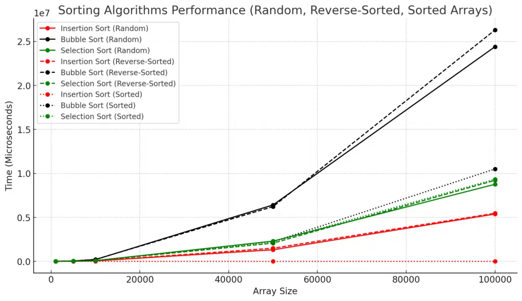
Let's present the results as graphs to understand the algorithms' behaviour better.

Analysis of Sorting Algorithm Performance Test

General Trends

• Bubble Sort is consistently the slowest across all input types and array sizes. Its quadratic time complexity (O(n²)) leads to significantly longer runtimes as the input size increases.
• Insertion Sort is generally faster than Bubble Sort, especially for smaller arrays and nearly sorted data. However, its performance degrades on large arrays, particularly with random or reverse-sorted input.
• Selection Sort sits between Bubble Sort and Insertion Sort in terms of speed. It remains slower than Insertion Sort on small datasets but outperforms Bubble Sort in most cases.

Performance on Random Arrays

• Bubble Sort performs the worst on random arrays. For larger array sizes like 50,000 and 100,000 elements, Bubble Sort requires over 24 million microseconds to sort the array, which is significantly slower than both Insertion and Selection Sort.
• Insertion Sort performs much better on random arrays, especially for smaller sizes like 1000, which only takes 607 microseconds compared to Bubble Sort's 1686 microseconds. However, as the array grows, its performance degrades to over 5 million microseconds for the 100,000-element array.
• Selection Sort has intermediate performance, taking longer than Insertion Sort but faster than Bubble Sort on random arrays.

Performance on Reverse-Sorted Arrays

• Bubble Sort again shows the slowest performance, taking the longest to sort reverse-sorted arrays. For the largest array size (100,000), it requires over 26 million microseconds.
• As expected, Insertion Sort is slower on reverse-sorted arrays than on random ones. However, it still significantly outperforms Bubble Sort. For example, at 100,000 elements, Insertion Sort takes around 5.4 million microseconds compared to Bubble Sort's 26 million.
• Selection Sort shows similar behavior to its performance on random arrays, being faster than Bubble Sort but slower than Insertion Sort.

Performance on Sorted Arrays

• Insertion Sort excels in this category. Insertion Sort has an O(n) best-case time complexity for already sorted arrays, making it extremely fast (3 microseconds for a 1000-element array and just 356 microseconds for a 100,000-element array).
• Bubble Sort does not perform nearly as well on sorted arrays, taking over 10 million microseconds to sort a 100,000-element sorted array. Its lack of optimization for already sorted data explains this performance.
• Selection Sort also fails to capitalize on sorted data, showing no significant performance boost. It behaves similarly to its performance on random arrays, with times of over 9 million microseconds for large arrays.

Key Takeaways

1. Insertion Sort excels on nearly sorted data
   • For sorted and almost sorted data, Insertion Sort outperforms Bubble Sort and Selection Sort by a wide margin. Its O(n) best-case time complexity allows it to sort arrays extremely quickly when minimal rearrangement is required.
2. Bubble Sort is consistently the slowest
   • Across all array types and sizes, Bubble Sort demonstrates the slowest performance. It struggles particularly with large arrays, making it an inefficient choice for anything beyond small or simple datasets.
3. Selection Sort is steady but not optimal
   • Selection Sort shows consistent but suboptimal performance. It performs better than Bubble Sort but is outpaced by Insertion Sort, especially on smaller and sorted datasets.
4. Larger array sizes widen the performance gap
   • The performance gap between these sorting algorithms becomes more pronounced as the array size increases. For 100,000-element arrays, the differences in performance are especially noticeable, with Bubble Sort taking over 24 million microseconds compared to Insertion Sort's 5 million microseconds on random data.
5. Choice of algorithm depends on input characteristics
   • If the input is likely to be sorted or nearly sorted, Insertion Sort is the best choice.
   • For other cases, both Insertion and Selection Sort can be used, but Bubble Sort should be avoided due to its poor performance.

Why Sorting Algorithm Performance Can Vary: Hardware and Memory Factors

The performance of sorting algorithms can vary significantly based on several hardware and system-related factors:

1. CPU Speed:
   • The CPU's processing power directly affects how quickly an algorithm can execute. Higher clock speeds and more CPU cores can allow faster sorting, especially for more complex algorithms like Bubble Sort, which involve many comparisons and swaps.
2. Memory and Cache:
   • Cache locality plays a vital role in algorithm performance. Algorithms like Insertion Sort, which access memory predictably and sequentially, may benefit from better cache utilization than Bubble Sort or Selection Sort, which may involve more scattered memory access.
   • Limited memory can lead to paging, where data is swapped between RAM and disk storage, significantly slowing down performance, especially for large arrays.
3. System Load:
   • Performance can be affected if the system is running other resource-intensive processes simultaneously, causing contention for CPU cycles or memory. This can lead to inconsistent results when benchmarking sorting algorithms.
4. Compiler Optimizations:
   • The compiler used to build the code can apply various optimization techniques (such as loop unrolling or instruction pipelining) to speed up the execution of sorting algorithms. Different optimization levels can result in faster or slower performance.

---

When to Use Insertion Sort

• Small datasets: For small arrays, the overhead of more advanced algorithms like Merge Sort or Quick Sort may not be worth it.
• Nearly sorted arrays: Insertion Sort performs particularly well on nearly sorted arrays, with a best-case time complexity of O(n).
• Stable sorting: Insertion Sort is stable, which is important if you need to preserve the relative order of elements with equal values.

---

How Insertion Sort is Used in TimSort

TimSort is a hybrid sorting algorithm that combines the advantages of Insertion Sort and Merge Sort. It was designed to be efficient on real-world data, often containing many ordered sequences (runs). One key strategy in TimSort is to use Insertion Sort for small subsections of the data.

Role of Insertion Sort in TimSort:

In TimSort, Insertion Sort is applied to small subsections of the data (called "runs") because it performs very efficiently on small datasets and nearly sorted data. These runs are either naturally occurring or created by the algorithm, typically of size 32 or 64. Due to its lower overhead, Insertion Sort is often faster than Merge Sort for such small runs.

Here’s how Insertion Sort is integrated into TimSort:

1. Divide the Data into Runs:
   • TimSort divides the array into small chunks (called runs), which are either already sorted or are sorted using Insertion Sort.
   • The size of these runs is generally between 32 and 64, which is optimal for Insertion Sort.
2. Use Insertion Sort to Sort the Runs:
   • Each run is individually sorted using Insertion Sort. Since Insertion Sort works well for small arrays and nearly sorted data, this step ensures that each run is efficiently sorted.
3. Merge the Sorted Runs Using Merge Sort:
   • After the runs are sorted, Merge Sort is used to combine them into a fully sorted array. Since Merge Sort performs well for merging larger datasets, it handles the merging of these small, sorted runs efficiently.

Why Use Insertion Sort in TimSort?

• Efficiency on Small Data: For small data sets or nearly sorted sequences, Insertion Sort is faster than more complex algorithms like Merge Sort.
• Adaptive Nature: Insertion Sort can take advantage of partially sorted data, making it the ideal candidate for sorting the small chunks or runs that TimSort relies on.
• Minimal Overhead: Insertion Sort's simple structure and minimal overhead make it a good fit for optimizing the early steps of TimSort.

Conclusion

Insertion Sort is simple and intuitive and works well for small datasets or nearly sorted data. While it may not be the fastest algorithm for large datasets, its elegance lies in its simplicity and its ability to work in place with minimal memory overhead.

You might want to consider Merge Sort or Quick Sort for more complex sorting needs, but for small data, Insertion Sort remains a solid choice.

Congratulations on reading to the end of this tutorial!

To implement Insertion Sort in Python, read the article: How to do Insertion Sort in Python.

For further reading on sorting algorithms in C++, go to the articles:

• How To Do Comb Sort in C++
• How To Do Quick Sort in C++
• How To Do Heap Sort in C++
• How To Do Merge Sort in C++
• Shell Sort in C++

For further exploration into Data Structures and Algorithms (DSA), please refer to the DSA page.

Have fun and happy researching!