How To Calculate Tukey’s Fences in R: Detecting Outliers in Your Data with Practical Examples

Tukey’s Fences is a statistical method used for outlier detection, offering a clear and effective way to identify data points that deviate significantly from the rest. Developed by John Tukey, this method applies a simple rule based on interquartile range (IQR) to flag potential outliers. In this article, we’ll explore how to calculate Tukey’s Fences and apply it to example datasets.

What is Tukey’s Fences?

Tukey’s Fences uses the interquartile range (IQR) to define outlier boundaries:

• The lower fence is calculated as \( Q_1 – 1.5 \times IQR \).
• The upper fence is calculated as \( Q_3 + 1.5 \times IQR \).

where:

• \( Q_1 \) is the first quartile (25th percentile),
• \( Q_3 \) is the third quartile (75th percentile), and
• \( IQR = Q_3 – Q_1 \), the interquartile range.

Data points outside these fences are considered mild outliers. A more extreme boundary, called the outer fence, is defined as:

\[ \text{Outer Fence} = Q_1 – 3 \times IQR \quad \text{and} \quad Q_3 + 3 \times IQR \]

Values beyond these outer fences are extreme outliers.

Calculating and Plotting Tukey’s Fences

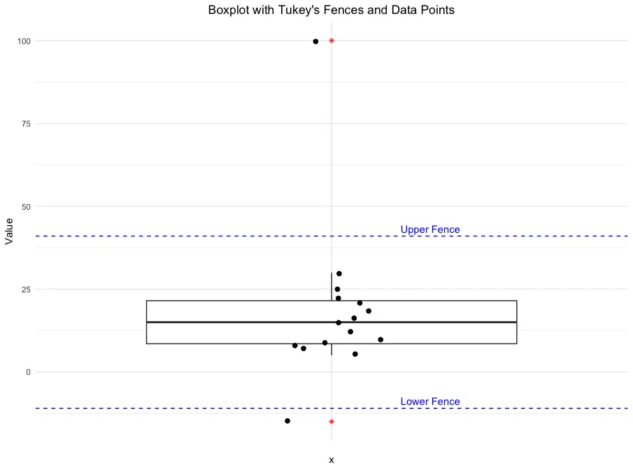
To calculate Tukey’s Fences in R, we start by computing the quartiles and interquartile range (IQR) of a dataset. We will also plot the data along with the calculated lower and upper fences, using a boxplot and individual points to visualize potential outliers. Here’s the code to perform these steps:

# Sample data
data <- c(5, 7, 8, 9, 10, 12, 15, 16, 18, 21, 22, 25, 30, 100, -15)

# Calculate Q1, Q3, and IQR
Q1 <- quantile(data, 0.25)
Q3 <- quantile(data, 0.75)
IQR_value <- IQR(data)

# Calculate fences
lower_fence <- Q1 - 1.5 * IQR_value
upper_fence <- Q3 + 1.5 * IQR_value

# Print the results
cat("Lower Fence:", lower_fence, "\n")
cat("Upper Fence:", upper_fence, "\n")

# Identify outliers
outliers <- data[data < lower_fence | data > upper_fence]
cat("Outliers: ", outliers, "\n")

# Load ggplot2 for plotting
library(ggplot2)

# Create a boxplot with points, showing fences as dashed lines
ggplot(data.frame(Value = data), aes(x = "", y = Value)) +
  geom_boxplot(outlier.colour = "red", outlier.shape = 8) +  # Boxplot
  geom_jitter(width = 0.1, aes(color = "Data Points"), size = 2) +  # Data points
  geom_hline(yintercept = lower_fence, linetype = "dashed", color = "blue") +  # Lower fence
  geom_hline(yintercept = upper_fence, linetype = "dashed", color = "blue") +  # Upper fence
  labs(title = "Boxplot with Tukey's Fences and Data Points",
       y = "Value") +
  theme_minimal() +
  theme(plot.title = element_text(hjust = 0.5))  +  # Centers the title
  annotate("text", x = 1.2, y = lower_fence, label = "Lower Fence", color = "blue", vjust = -0.5) +
  annotate("text", x = 1.2, y = upper_fence, label = "Upper Fence", color = "blue", vjust = -0.5) +
  scale_color_manual(name = "", values = c("Data Points" = "black")) +
  theme(legend.position = "none")  # Hides the legend for cleaner display

This code calculates the lower and upper fences, identifies outliers, and then uses ggplot2 to create a boxplot, adding individual data points as jittered points for better visibility. The lower and upper fences are shown as dashed horizontal lines, with annotations to label each fence. This combined plot helps us visualize data distribution, identify outliers, and understand Tukey’s Fences in a practical context.

Lower Fence: -11
Upper Fence: 41
Outliers:  100 -15

Assumptions and Limitations of Tukey’s Fences

Assumptions: Tukey’s Fences assumes that the data is approximately symmetric and does not have heavy tails (extreme skewness or kurtosis). It works best with distributions that are fairly well-behaved and relatively symmetric around the median, such as normal or mildly skewed distributions.

This method relies on the interquartile range (IQR) to identify outliers, which inherently assumes that most of the data falls within a predictable range. Therefore, Tukey’s Fences might be less effective when used on highly skewed data or datasets with an excessive number of outliers.

Limitations: While Tukey’s Fences is a simple and effective approach, it has limitations. In cases where data is skewed, the calculated fences may not appropriately capture outliers, either missing significant outliers in the tails or misidentifying normal observations as outliers.

Another limitation is its sensitivity to the choice of multiplier (usually 1.5 for mild outliers and 3 for extreme outliers). For certain datasets, adjusting these multipliers may be necessary to capture relevant outliers accurately, especially in financial or biological data where distributions can deviate significantly from normality.

In summary, while Tukey’s Fences is useful for initial outlier detection, it should be applied with an understanding of the data’s distribution and in conjunction with other methods when analyzing data with irregular shapes or extreme values.

Conclusion

Tukey’s Fences is a valuable tool for identifying outliers in your dataset. By using the interquartile range, this method creates a simple and effective rule for flagging data points that deviate significantly from the norm. Whether analyzing financial transactions, biological measurements, or survey data, Tukey’s Fences provides a robust framework for detecting anomalies. Remember, outliers aren’t always errors—they could represent important, unexpected insights. Treat outliers carefully and in the context of your specific analysis goals.

Try the Tukey’s Fences Outlier Detector

If you’d like to quickly identify outliers in your own data, try our Tukey’s Fences Outlier Detector on the Research Scientist Pod.

Have fun and happy researching!