Understanding the Central Limit Theorem (CLT) with Practical Examples

The Central Limit Theorem (CLT) is a foundational concept in statistics, asserting that the sampling distribution of the sample mean will approximate a normal distribution as the sample size grows, regardless of the original data distribution. This guide explains CLT through a step-by-step example, beginning with a uniformly distributed dataset.

Introduction to the Central Limit Theorem

In statistics, the CLT bridges individual data and population parameters. It allows us to make inferences about the population from a sample by demonstrating that, with a large enough sample size, the distribution of sample means becomes normally distributed. This principle supports many inferential statistical methods, making it one of the most widely used theorems in the field.

The Formula for the Central Limit Theorem

The Central Limit Theorem states that for a population with mean \( \mu \) and standard deviation \( \sigma \), the distribution of sample means (with sufficiently large sample size \( n \)) will approximate a normal distribution. This sampling distribution has:

\[ \text{Mean of the Sampling Distribution (Expected Value)} = \mu \]

\[ \text{Standard Deviation of the Sampling Distribution (Standard Error)} = \frac{\sigma}{\sqrt{n}} \]

Thus, the standardized form of the sample mean \( \bar{X} \) can be written as:

\[ Z = \frac{\bar{X} – \mu}{\sigma / \sqrt{n}} \]

where \( Z \) follows a standard normal distribution, \( N(0,1) \).

Properties of the Central Limit Theorem

The CLT has several important properties that make it powerful in statistical applications:

• Normality of Sample Means: No matter the shape of the original population distribution, the distribution of sample means will approach normality as the sample size increases.
• Sample Size Requirement: A larger sample size yields a better approximation to normality. Generally, a sample size of \( n \geq 30 \) is considered sufficient for the CLT to hold, though smaller samples may suffice for populations that are already symmetric.
• Unbiased Estimation: The mean of the sampling distribution is equal to the population mean, \( \mu \), ensuring that sample means are unbiased estimators of the population mean.
• Standard Error: The spread of the sampling distribution, called the standard error, decreases as the sample size increases, following \( \frac{\sigma}{\sqrt{n}} \). This property implies that larger samples provide more precise estimates.

Example: Starting with a Uniformly Distributed Sample

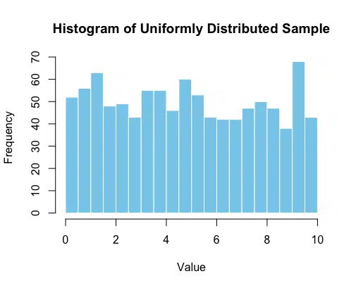
To demonstrate the CLT, let’s start with a uniformly distributed dataset, where all values have an equal likelihood. Here’s how we can generate and plot such a sample in R:

# Generate a uniform sample
set.seed(42)  # for reproducibility
uniform_sample <- runif(1000, min = 0, max = 10)

# Plot the histogram
hist(uniform_sample,
     main = "Histogram of Uniformly Distributed Sample",
     xlab = "Value",
     ylab = "Frequency",
     col = "skyblue",
     border = "white",
     breaks = 20)

This histogram shows the flat (or “uniform”) distribution where each value within the range [0, 10] has an approximately equal probability of occurring.

Building the Sampling Distribution of the Mean

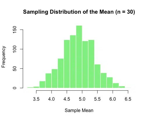
Next, we’ll take samples from our uniformly distributed data, calculate the sample means, and observe how they form a distribution. As per the CLT, as the sample size and number of samples increase, this distribution will converge to a normal shape.

# Define parameters for sampling
sample_size <- 30  # size of each sample
n_samples <- 1000  # number of samples

# Generate sample means
sample_means <- replicate(n_samples, mean(sample(uniform_sample, sample_size, replace = TRUE)))

# Plot the histogram of sample means
hist(sample_means,
     main = "Sampling Distribution of the Mean (n = 30)",
     xlab = "Sample Mean",
     ylab = "Frequency",
     col = "lightgreen",
     border = "white",
     breaks = 20)

This histogram illustrates the distribution of sample means. Although the original dataset was uniformly distributed, the sampling distribution of the mean begins to approximate a normal distribution.

Now that we’ve examined the distribution of sample means and how it centers around the population mean, let’s explore the behavior of sample variances. Sample variance is calculated within each sample and provides an estimate of the population variance. Like the sample mean, sample variance is also influenced by the sample size and is expected to fluctuate around the population variance. However, the distribution of sample variances behaves slightly differently, as it does not perfectly mirror the properties of sample means. We’ll now delve into these characteristics to understand the implications of sample variance in statistical inference.

Understanding Sample Variance Distributions

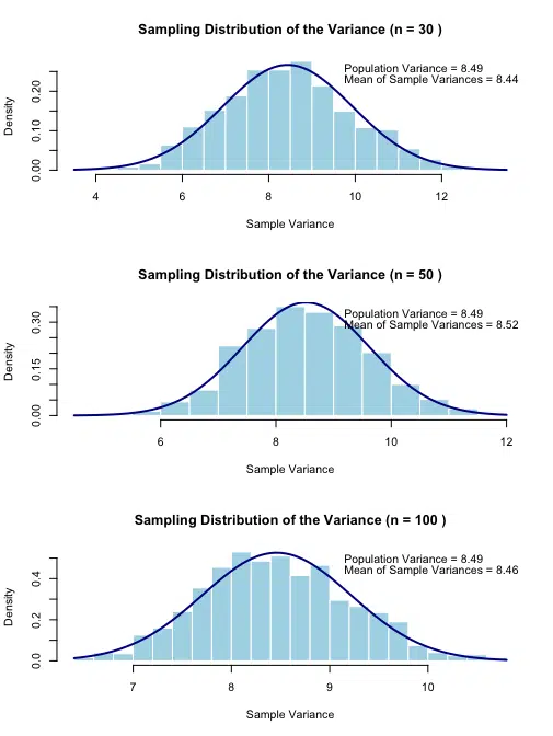
To better understand how sample variances relate to population variance, let's explore how increasing the sample size affects the distribution of sample variances. We'll examine how sample variances from different sample sizes distribute around the true population variance, and how the spread of these sample variances changes with sample size.

Code Implementation

# Generate a uniform sample
set.seed(42)  # for reproducibility
uniform_sample <- runif(1000, min = 0, max = 10)

# Calculate population parameters
population_mean <- mean(uniform_sample)
population_variance <- var(uniform_sample)

# Print the population mean and variance
cat("Population Mean:", round(population_mean, 2), "\n")
cat("Population Variance:", round(population_variance, 2), "\n\n")

# Function to plot the histogram with a normal distribution curve and print sample stats
plot_sample_vars <- function(sample_size) {
    # Generate sample means and sample variances
    sample_means <- replicate(n_samples, mean(sample(uniform_sample, sample_size, replace = TRUE)))
    sample_vars <- replicate(n_samples, var(sample(uniform_sample, sample_size, replace = TRUE)))

    # Calculate mean and variance of sample variances
    mean_sample_var <- mean(sample_vars)
    var_sample_var <- var(sample_vars)

    # Calculate mean and variance of sample means
    mean_sample_mean <- mean(sample_means)
    var_sample_mean <- var(sample_means)

    # Expected variance of sample means
    expected_var_sample_mean <- population_variance / sample_size

    # Plot the histogram of sample variances
    hist(sample_vars,
         probability = TRUE,
         main = paste("Sampling Distribution of the Variance (n =", sample_size, ")"),
         xlab = "Sample Variance",
         ylab = "Density",
         col = "lightblue",
         border = "white",
         breaks = 20)

    # Overlay a normal distribution curve for sample variances
    curve(dnorm(x, mean = mean_sample_var, sd = sqrt(var_sample_var)),
          add = TRUE,
          col = "darkblue",
          lwd = 2)

    # Print sample statistics
    cat("Sample Size:", sample_size, "\n")
    cat("Mean of Sample Means:", round(mean_sample_mean, 2), "\n")
    cat("Variance of Sample Means:", round(var_sample_mean, 4), "\n")
    cat("Expected Variance of Sample Means:", round(expected_var_sample_mean, 4), "\n")
    cat("Mean of Sample Variances:", round(mean_sample_var, 2), "\n")
    cat("Variance of Sample Variances:", round(var_sample_var, 4), "\n\n")

    # Display population and sample statistics in a legend
    legend("topright",
           legend = c(
               paste("Population Mean =", round(population_mean, 2)),
               paste("Mean of Sample Means =", round(mean_sample_mean, 2)),
               paste("Population Variance =", round(population_variance, 2)),
               paste("Mean of Sample Variances =", round(mean_sample_var, 2)),
               paste("Expected Variance of Sample Means =", round(expected_var_sample_mean, 4))
           ),
           bty = "n")
}

# Define parameters for sampling
n_samples <- 1000  # number of samples

# Plot the distributions and print sample statistics for different sample sizes
par(mfrow = c(3, 1))  # Arrange plots in a 3-row layout
plot_sample_vars(30)
plot_sample_vars(50)
plot_sample_vars(100)

Sample Size: 30
Mean of Sample Means: 4.87
Variance of Sample Means: 0.265
Expected Variance of Sample Means: 0.2831
Mean of Sample Variances: 8.56
Variance of Sample Variances: 2.0964

Sample Size: 50
Mean of Sample Means: 4.88
Variance of Sample Means: 0.1686
Expected Variance of Sample Means: 0.1699
Mean of Sample Variances: 8.53
Variance of Sample Variances: 1.1657

Sample Size: 100
Mean of Sample Means: 4.87
Variance of Sample Means: 0.089
Expected Variance of Sample Means: 0.0849
Mean of Sample Variances: 8.51
Variance of Sample Variances: 0.621

Understanding the Visualization

The code above creates three histograms showing the distribution of sample variances for different sample sizes (n=30, 50, and 100). Each plot includes:

• A histogram of sample variances calculated from repeated sampling
• An overlaid normal distribution curve
• The true population variance for reference
• The mean of the sample variances

Key observations from these visualizations:

1. Convergence of Mean: The mean of the sample variances should be close to the population variance for all sample sizes, demonstrating that the sample variance is an unbiased estimator of the population variance.
2. Reduction in Spread: As the sample size increases, the distribution of sample variances becomes narrower, indicating that individual sample variances become more reliable estimates of the population variance.
3. Shape of Distribution: The distribution of sample variances tends to become more symmetric and normal-like as the sample size increases, though this convergence is slower than for sample means.

These visualizations help demonstrate that while individual sample variances may differ from the population variance, their average converges to the true population variance, and their variability decreases with larger sample sizes.

Understanding Sampling Mean and Variance vs. Population Mean and Variance

To fully understand the Central Limit Theorem, it's essential to differentiate between the population mean and variance and the sampling mean and variance. These concepts reveal why the CLT is a powerful tool for drawing insights about a population from sample data.

Population Mean and Variance

The population mean and population variance describe the overall distribution of data points in the entire population. They are theoretical parameters that provide insight into the central tendency and spread of all possible values in the population.

• Population Mean (\( \mu \)): The population mean is the average of all values in the population. It represents the central point of the distribution. \[ \mu = \frac{1}{N} \sum_{i=1}^N X_i \] where \( N \) is the total number of observations in the population, and \( X_i \) are the individual data points.
• Population Variance (\( \sigma^2 \)): The population variance is the average squared deviation of each data point from the population mean. It measures the spread of values in the population. \[ \sigma^2 = \frac{1}{N} \sum_{i=1}^N (X_i - \mu)^2 \] A larger population variance indicates a wider spread of values, while a smaller variance indicates that the values are closer to the mean.

In real-world scenarios, we rarely have access to the entire population. Instead, we work with samples, using their statistics to estimate the population parameters.

Sample Mean and Variance

The sample mean and sample variance are calculated from a subset of the population, known as a sample. These metrics provide estimates of the population parameters but are subject to sampling variability.

• Sample Mean (\( \bar{X} \)): The sample mean is the average of values within a single sample, and it serves as an estimate of the population mean. \[ \bar{X} = \frac{1}{n} \sum_{i=1}^n x_i \] where \( n \) is the sample size, and \( x_i \) are the individual values in the sample.
• Sample Variance (\( s^2 \)): The sample variance is calculated using (n-1) in the denominator to provide an unbiased estimate of the population variance. \[ s^2 = \frac{1}{n - 1} \sum_{i=1}^n (x_i - \bar{X})^2 \]

Key Relationships and Properties

1. Sample Mean Distribution:
   • The distribution of sample means centers around the population mean
   • Its variance equals the population variance divided by n: \( \text{Var}(\bar{X}) = \frac{\sigma^2}{n} \)
   • As sample size increases, this distribution becomes more normal (CLT)
2. Sample Variance Properties:
   • Individual sample variances vary randomly around the population variance
   • The mean of many sample variances approaches the population variance
   • The spread of sample variances decreases with larger sample sizes
3. Important Distinctions:
   • Sample variance ≠ Variance of sample means
   • Sample variances estimate population variance (σ²)
   • Variance of sample means equals σ²/n

Practical Implications

Understanding these relationships helps us:

• Properly interpret sample statistics
• Recognize why larger samples provide more reliable estimates
• Understand why sample variance uses (n-1) in its denominator
• Avoid confusion between sample variance and variance of sample means

These concepts form the foundation for statistical inference and help explain why we can make reliable conclusions about populations using sample data, even when the population's distribution is unknown.

Use Cases for the Central Limit Theorem

The Central Limit Theorem is applied across various domains and is essential for enabling many statistical techniques:

• Estimating Population Parameters: CLT allows us to estimate the population mean and variance from sample data, especially in cases where sampling the entire population is impractical.
• Constructing Confidence Intervals: The normality of sample means enables the construction of confidence intervals, allowing for reliable inferences about population parameters.
• Hypothesis Testing: Many hypothesis tests (e.g., t-tests) assume normality in the sampling distribution. CLT provides the theoretical foundation to apply these tests even if the underlying data isn’t normally distributed.
• Quality Control: In manufacturing, sample means of product measurements are tracked to ensure they meet quality standards. The CLT ensures these sample averages are normally distributed, enabling accurate quality checks.
• Financial Modeling: Financial analysts use the CLT to make predictions about stock returns by assuming normality in the distribution of average returns, helping in portfolio optimization and risk management.

Conclusion

The Central Limit Theorem is a cornerstone of statistical theory, showing that the sampling distribution of the mean will approach normality as sample sizes increase. Through the CLT, we gain powerful tools for estimating and testing population parameters from sample data, supporting critical statistical methods and analyses.

Try the Central Limit Theorem Simulator

Try our Central Limit Theorem Simulator to see CLT in action with your own data. Have fun and happy researching!