An Introduction to the Sigmoid Function

This article will go through the sigmoid function formula, sigmoid function as an activation function, the ways to implement the sigmoid function in Python, and a brief history of the origins and applications of the sigmoid function. After reading through this article, you will know:

• The sigmoid function formula
• How to calculate the derivate of the sigmoid function
• The properties of the sigmoid function which make it useful for machine learning
• The limitations of the sigmoid function
• How to implement the sigmoid funcion in Python using the NumPy and SciPy libraries
• The history of the sigmoid function

What is the Sigmoid Function?

A sigmoid function is a mathematical function with a characteristic S-shaped curve. There are several types of sigmoid functions, including the logistic, the hyperbolic tangent and the arctangent functions. Sigmoid functions are widely used in machine learning, particularly deep learning, where they serve as activation functions in an artificial neural network. The use of activation functions is similar to the activation potential in biological neural networks.

We can use sigmoid functions to convert a real number to a probability for machine learning applications. We can place a sigmoid function at the end of a machine learning model to convert the model’s output to a probability score. Probability scores are helpful for classification. For example, logistic regression for two-class classification converts several real number inputs into a probability. The conversion to a probability involves the logistic function at the final stage of a logistic regression model.

Sigmoid Function Formula

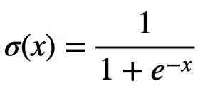
The sigmoid function, denoted by is given by:

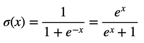
We also can express the sigmoid function mathematically as:

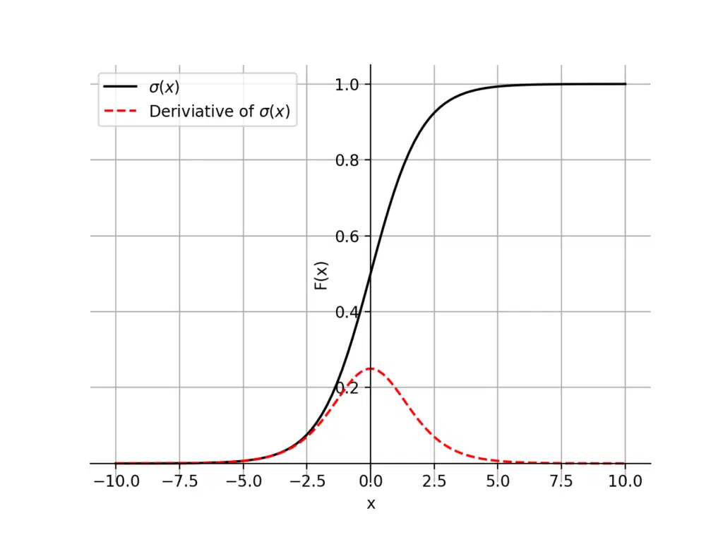
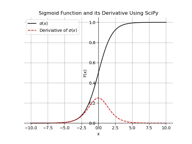
The graph of the sigmoid function is a characteristic S-shaped curve as shown below in black. The figure also shows the derivative of the sigmoid function in red.

Properties of the Sigmoid Function

The sigmoid function has many interesting properties:

• The domain of the functions is from negative infinity to infinity, ()
• As x tends to negative infinity, the sigmoid function tends to 0. As x tends to infinity, the sigmoid function tends to 1. Therefore, the range of the sigmoid function is: (0, +1)
• The function is monotonically increasing, meaning as x increases the function increases for all real x values.
• You can differentiate the sigmoid function everywhere in its domain
• The function is continuous everywhere
• You can calcualte the function’s value across a small range of values, for example [-10, 10]. For values lower -10, the function is near zero and for values higher than +10, the function is near one.

Derivative of the Sigmoid Function

Artificial neural networks can use backpropagation for supervised learning. Backpropagation, which is short for backward propagation of errors, uses gradient descent. Given an artificial neural network and an error function, gradient descent calculates the gradient of the error function with respect to the neural network’s weights. The gradient calculation proceeds backwards through the network, with the gradient of the final layer of weights calculated first and the gradient of the first layer of weights calculated last. The error function includes the activation function. Therefore it is useful to know the derivative of the activation function. Let’s look at how to calculate the derivative of the sigmoid function:

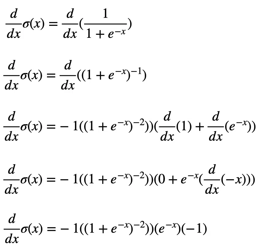
Now that we have seen how to compute the derivative of the sigmoid function, we can simplify the terms:

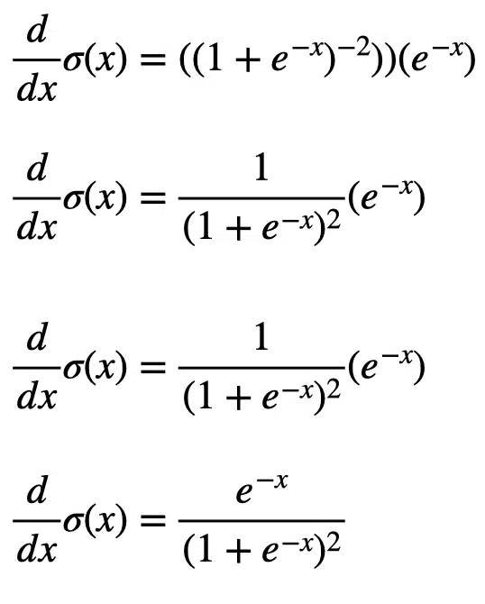
This result is simple, but we can separate the right-hand side of the equation subtract one from the second term to get something different:

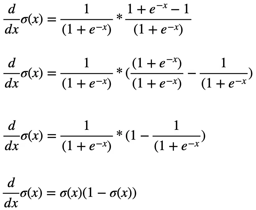
The final result elegantly shows that the derivative of the sigmoid function is equal to the sigmoid function multiplied by one minus the sigmoid function.

Sigmoid Function As a Squashing Function

Squashing functions convert an unbounded space to a bounded probability space in machine learning. We can call the sigmoid function a squashing function because its domain is the set of all real numbers, and its range is (0, 1). Therefore, if we have any number between and , the output from the sigmoid function will always be between 0 and 1. The sigmoid function can squash the output from the final layer of a neural network to the range of (0, 1), allowing us to interpret the model’s model’s final outputs as probabilities.

Sigmoid Function as an Activation Function in Neural Networks

An activation function is a simple function that receives inputs and outputs values within a defined range. In neural networks, we pass a weighted sum of inputs through an activation function, which outputs a bounded value to send to the next layer of neurons or as the final output. Activation functions determine which neuron to activate in a neural network.

If we use a linear activation function in a neural network, this model can only learn linearly separable problems. Non-linear activation functions enable neural networks to capture nonlinearity in data and learn complex decision functions.

When the activation function is a sigmoid function, the neuron’s output will always be between 0 and 1 and will be a non-linear function of the weighted sum of inputs. A neuron that employs a sigmoid function as an activation function is called a sigmoid unit. Below is a visualization of a sigmoid unit in a neural network.

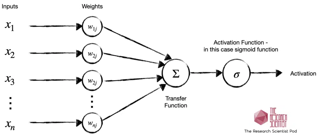
The artificial neuron is analogous to the biological neuron. To learn more about the artificial neural networks and their connection to biological neurons, go to “The History of Machine Learning” and “The History of Reinforcement Learning“.

Why is the Sigmoid Function Important for Neural Networks?

The sigmoid function provides a non-linear activation function, which enables models that use it to learn non-linearly separable problems.

For neural networks, we can only use a monotonically increasing activation, which rules out functions such as sine and cosine. However, sigmoid functions are monotonically increasing and are well suited to neural networks.

Activation functions need to provide a definition everywhere in the real number space and be continuous. The sigmoid function is continuous and has a negative and positive infinity domain.

Activation functions need to be differentiable over the entire real number space. We can see from calculating the derivative of the sigmoid function that it can provide a definition for all real numbers.

The sigmoid function is suitable for gradient descent in backpropagation because of the above characteristics. We can express its derivative in terms of itself, which makes error propagation easy to perform when training a neural network using backpropagation.

What are the Limitations of the Sigmoid Function?

The sigmoid function saturates, which means for small and large values of x, the functions is 0 and 1, respectively. The function is only really sensitive around the midpoint or 0.5. The limited sensitivity coupled with saturation means any meaningful information provided as input can be lost. Once the function is saturated, it becomes challenging for the learning algorithm to continue to update the weights to improve model performance.

Sigmoid functions suffer from the vanishing gradient problem. This problem occurs during backpropagation. As we update the weights, the gradients we transfer back to the earlier layers become exponentially smaller. At some points, the updating gradients almost vanish or become very close to zero, halting the network’s ability to learn. We can refer to the derivative of the sigmoid function: . Since is always less than 1, the derivative will always involve multiplying two values less than one, which will result in an even smaller value. With the repetitive computation of the gradient of the sigmoid function, the value will approach zero. Vanishing gradients prevent us from building deep neural networks.

The sigmoid function is not zero-centred. Therefore when we perform gradient descent, the updates will either be all positive or negative, and the weights will move in the same direction. Consequently, the gradient updates will take on a “zig-zag” path, which is less efficient than taking the optimal path.

We want to have a certain degree of model sparsity when training neural networks. The fewer neurons there are, the sparser the model is and the faster it will converge to an optimal value. Sigmoid functions produce non-sparse models because their neurons always produce an output value between [0, 1], but never a true zero value. Therefore, we cannot remove specific neurons that are not effective, preventing us from reducing model complexity.

The sigmoid functions require an exponential calculation, which is computationally more expensive than linear functions.

We can solve the problems of saturation, vanishing gradient, model complexity and computation expense with the Rectified Linear Unit (ReLU) activation function. We can solve the problem of non-zero centering with the hyperbolic tangent function (tanh), though the TanH function still suffers the other limitations.

How to Implement the Sigmoid Function In Python

In this section, we will learn how to calculate the sigmoid function using the SciPy and NumPy Python libraries. To learn more about Python libraries for data science and machine learning, go to the article “Top 12 Python Libraries for Data Science and Machine Learning“.

Implement the Sigmoid Function in Python Using the SciPy Library

The SciPy library version of the sigmoid function is called expit(). Let’s use the expit() function to calculate the sigmoid function and its derivative for a range of x-values between -10 and 10. We can use the simplified derivative term from the earlier section. We will also create a plotting function that plots the sigmoid function and its derivative in the range [-10, 10].

import numpy as np

import matplotlib.pyplot as plt

from scipy.special import expit

def scipy_sigmoid(x):

    sig = expit(x)

    return sig

def plot_function(x, y, dy, name):

    ticks = [0.2, 0.4, 0.6, 0.8, 1.0]

    ax = plt.gca()

    ax.spines['top'].set_color('none')

    ax.spines['left'].set_position('zero')

    ax.spines['right'].set_color('none')

    ax.spines['bottom'].set_position('zero')

    plt.plot(x, y, color='k', label='$\sigma(x)$')

    plt.plot(x, dy, color='r', linestyle='dashed', label='Deriviative of $\sigma(x)$')

    plt.grid(True)

    plt.legend()

    plt.xlabel('x')

    plt.ylabel('F(x)')

    plt.title('Sigmoid Function and its Derivative Using SciPy')

    plt.savefig('figs/sigmoid_function_using_'+name+'.png')

    plt.close()

if __name__ == '__main__':

    # Define x values

    x = np.linspace(-10, 10, 100)

    # Calculate sigmoid function for x values

    y = scipy_sigmoid(x)

    # Calculate derivate of sigmoid function

    dy = y * (1 - y)

    # Plot function and its derivative

    plot_function(x, y, dy, 'scipy')                                      

The expit() method is slower than the numpy implementation. However, the advantage of the expit() method is it can automatically handle various types of inputs like lists and numpy arrays. Let’s look at an example of using the expit() function on a numpy array:

from scipy.special import expit

import numpy as np

an_array = np.array([0.15, 0.4, 0.5, 0.9, 0.2])

sig = expit(an_array)

print(sig)

[0.53742985 0.59868766 0.62245933 0.7109495  0.549834  ]

Implement the Sigmoid Function in Python Using the numpy.exp() Method

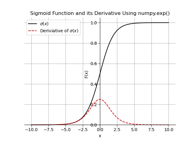
The sigmoid function has an exponential term. We can use numpy.exp() to calculate the sigmoid function. Let’s calculate the sigmoid function and its derivative for a range of x-values between -10 and 10. We can use the simplified derivative term from the earlier section. We will use the same plotting function as in the SciPy example to both the sigmoid function and its derivative in the range [-10, 10].

import numpy as np

import matplotlib.pyplot as plt

def numpy_sigmoid(x):

    z = np.exp(-x)

    sig = 1 / (1 + z)

    return sig

def plot_function(x, y, dy, name):

    ticks = [0.2, 0.4, 0.6, 0.8, 1.0]

    ax = plt.gca()

    ax.spines['top'].set_color('none')

    ax.spines['left'].set_position('zero')

    ax.spines['right'].set_color('none')

    ax.spines['bottom'].set_position('zero')

    plt.plot(x, y, color='k', label='$\sigma(x)$')

    plt.plot(x, dy, color='r', linestyle='dashed', label='Deriviative of $\sigma(x)$')

    plt.grid(True)

    plt.legend()

    plt.xlabel('x')

    plt.ylabel('F(x)')

    plt.savefig('figs/sigmoid_function_using_'+name+'.png')

    plt.close()

if __name__ == '__main__':

    # Define x values

    x = np.linspace(-10, 10, 100)

    # Calculate sigmoid function for x values

    y = numpy_sigmoid(x)

    # Calculate derivate of sigmoid function

    dy = y * (1 - y)

    # Plot function and its derivative

    plot_function(x, y, dy, 'numpy')

How to Use the PyTorch Sigmoid Function

The first way to apply the sigmoid in PyTorch is to use the torch.sigmoid() function:

import torch

torch.manual_seed(1)

x = torch.randn((4, 4, 4))

y = torch.sigmoid(x)

print(y.min(), y.max())

tensor(0.0345) tensor(0.9135)

The second way is to create an object of the torch.nn.Sigmoid() class and then calling the object.

import torch

class Model(torch.nn.Module):

    def __init__(self, input_dim):

        super().__init__()

        self.linear = torch.nn.Linear(input_dim, 1)

        self.activation = torch.nn.Sigmoid()

    def forward(self, x):

        x = self.linear(x)

        return self.activation(x)

torch.manual_seed(1)

model = Model(4)

x = torch.randn((10, 4))

y = model(x)

print(y.min(), y.max())

tensor(0.2182, grad_fn=<MinBackward1>) tensor(0.5587, grad_fn=<MaxBackward1>)

The History of the Sigmoid Function

The first appearance of the logistic function was in a series of three papers by Pierre Verhulst between 1838 and 1847, who devised it as a model for population growth. The logistic function adjusts the exponential growth model to account for the fact that population growth is ultimately self-limiting and does not increase exponentially forever. The logistic function models the slowing down of population growth, which occurs when a population begins to exhaust its resources. The initial stage of growth is approximately exponential, then as saturation begins or resources deplete, the growth slows to linear, then at maturity, the growth stops.

Throughout the 19th and centuries, biologists and other scientists used the sigmoid function to model population growth of various phenomena, including tumor growth in medicine to animal populations in ecology.

The use of sigmoid functions in artificial networks led to groundbreaking research, including Yann LeCun’s convolutional neural network LeNet, which uses the TanH function and can recognize handwritten digits to a practical level of accuracy.

In 1943, Warren McCulloch and Walter Pitts developed an artificial neural network model with a hard cutoff activation function. Each neuron outputs a value of 1 or 0 depending on whether its input is above or below a certain threshold.

In 1972, the biologists Hugh Wilson and Jack Crown at the University of Chicago developed the Wilson-Cowan model to model biological neurons. The model describes a neuron sending a signal to another neuron if it receives an input greater than its activation potential. The scientists chose the logistic sigmoid function to model the activation of a neuron as a function of a stimulus.

The adaptation of the sigmoid function to artificial neural networks started in the 1970s. In 1998, Yann Lecun chose the tanh function as the activation function for his convolutional neural network LeNet, producing groundbreaking results. LeNet was the first model to recognize handwritten digits to a high level of accuracy.

As described earlier, the sigmoid function has several limitations. As a result, deep learning has moved from sigmoid functions for activation functions in favor of the ReLU. The ReLU function is computationally cheap, does not suffer from the limitations of the sigmoid function and provides the necessary nonlinearity to construct and train deep neural networks.

Summary

Congratulations on reading to the end of this article. The sigmoid function is an elegant piece of mathematics with roots in modeling population growth and applications in machine learning and deep learning. In this article, you have gone through the properties of the sigmoid function, which makes it so exciting and valuable in machine learning and calculating the function in Python. You now know the limitations of the sigmoid function and the alternatives when training deep neural networks.

Go to the online courses page: Machine Learning to learn more about machine learning and deep learning.

Have fun and happy researching!