This tutorial will go through adding the regression line equation and R-squared to a plot in R with code examples.
Table of contents
What is the Regression Equation?
Linear regression is the statistical method of finding the relationship between two variables by fitting a linear equation to observed data.
One of the two variables is considered the explanatory variable, and the other is the response variable. A linear regression line has an equation called the regression equation, which takes the form Y = a +bX, where X is the explanatory variable and Y is the dependent variable. The gradient of the line is b, and a is the intercept (the value of y when x = 0)
You can use our free calculator to fit a linear regression model to predictor and response values.
What is the R-Squared Value?
When we fit a linear regression model to data, we need a value to tell us how well the model fits the data, and the R-square value does this for us.
We can define R-squared as the percentage of the response variable variation explained by the linear model.
R-squared is always between 0 and 1 or 0% and 100% where:
- 0 indicates that the model explains none of the variability of the response data around its mean.
- 1 indicates that the model explains all of the variability of the response data around its mean.
Generally, we can say that the higher the R-squared value, the better the linear regression model fits to the data. However, not all low R-squared values are intrinsically bad and not all R-squared values are intrinsically good.
Example: Using ggpubr
Let’s look at an example of fitting a linear regression model to some data and obtaining the regression equation and R-squared.
Create Data
We will use the built-in mtcars dataset. We can look at the available features in the dataset using the head() function:
head(mtcars)
   mpg cyl disp  hp drat    wt  qsec vs am gear carb
Mazda RX4         21.0   6  160 110 3.90 2.620 16.46  0  1    4    4
Mazda RX4 Wag     21.0   6  160 110 3.90 2.875 17.02  0  1    4    4
Datsun 710        22.8   4  108  93 3.85 2.320 18.61  1  1    4    1
Hornet 4 Drive    21.4   6  258 110 3.08 3.215 19.44  1  0    3    1
Hornet Sportabout 18.7   8  360 175 3.15 3.440 17.02  0  0    3    2
Valiant           18.1   6  225 105 2.76 3.460 20.22  1  0    3    1
We can see there are 11 features. We will choose miles-per-gallon (mpg) and weight (wt) as we are interested in the relationship between fuel efficiency and weight. We can see the values for each feature using the dollar-sign operator:
mtcars$wt
[1] 2.620 2.875 2.320 3.215 3.440 3.460 3.570 3.190 3.150 3.440 3.440 4.070 3.730 3.780
[15] 5.250 5.424 5.345 2.200 1.615 1.835 2.465 3.520 3.435 3.840 3.845 1.935 2.140 1.513
[29] 3.170 2.770 3.570 2.780
mtcars$mpg
 [1] 21.0 21.0 22.8 21.4 18.7 18.1 14.3 24.4 22.8 19.2 17.8 16.4 17.3 15.2 10.4 10.4
[17] 14.7 32.4 30.4 33.9 21.5 15.5 15.2 13.3 19.2 27.3 26.0 30.4 15.8 19.7 15.0 21.4
We can see if there is a linear relationship between the two variables by plotting as follows:
install.packages("ggplot2")
library(ggplot2)

ggplot(data=mtcars, aes(x=wt, y=mpg)) +
geom_point()
If you do not have ggplot2 installed, you must use the install.packages("ggplot2") command. Otherwise, you can omit it.
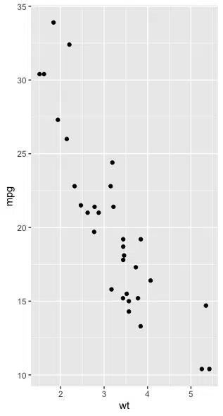
We can see that there is a linear relationship between mpg and wt.
Plot Data and Add Regression Equation
Next, we will install and load ggpubr to use the stat_regline_equation() function:
install.packages("ggpubr")
library(ggpubr)
Then we create the plot with the regression line and the regression equation as follows:
ggplot(data=mtcars, aes(x=wt, y=mpg)) +
geom_smooth(method="lm") +
geom_point() +
stat_regline_equation(label.x=4, label.y=30)
geom_smooth adds a line of best fit using linear regression and confidence bands in grey. stat_regline_equation adds a regression line to the plot.
The parameters label.x and label.y specify the x and y coordinates for the regression equation on the plot.
Let’s run the code to see the result:
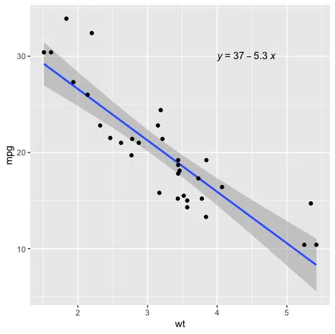
The fitted regression equation is
y = 37 - 5.3 * (x)
Where y is mpg and x is wt.
Plot Data and Add Regression Equation and R-Squared
We can add the R-squared value using the stat_cor() function as follows:
library(ggplot2)
library(ggpubr)

ggplot(data=mtcars, aes(x=wt, y=mpg)) +
geom_smooth(method="lm") +
geom_point() +
stat_regline_equation(label.x=4, label.y=30) +
stat_cor(aes(label=..rr.label..), label.x=4, label.y=28)

The R-squared value for this model is 0.75.
We can also find the parameters of the regression equation by using the lm() function as follows:
fit <- lm(mpg ~ wt, data = mtcars)
The tilde symbol ~ means “explained by”, which tells the lm() function that mpg is the response variable and wt is the explanatory variable. We can get the coefficients and R-Squared using summary() as follows:
summary(fit)
Call:
lm(formula = mpg ~ wt, data = mtcars)

Residuals:
    Min      1Q  Median      3Q     Max
-4.5432 -2.3647 -0.1252  1.4096  6.8727

Coefficients:
            Estimate Std. Error t value Pr(>|t|)
(Intercept)  37.2851     1.8776  19.858  < 2e-16 ***
wt           -5.3445     0.5591  -9.559 1.29e-10 ***
---
Signif. codes:
0 ‘***’ 0.001 ‘**’ 0.01 ‘*’ 0.05 ‘.’ 0.1 ‘ ’ 1

Residual standard error: 3.046 on 30 degrees of freedom
Multiple R-squared:  0.7528,	Adjusted R-squared:  0.7446
F-statistic: 91.38 on 1 and 30 DF,  p-value: 1.294e-10
We can see the estimated intercept is 37.3, and the gradient is -5.3, matching what we saw on the plot. The Multiple R-squared value is 0.75, which matches what we saw on the plot.
Summary
Congratulations on reading to the end of this tutorial!
For further reading on plotting in R, go to the articles:
- How to Place Two Plots Side by Side using ggplot2 and cowplot in R
- How to Download and Plot Stock Prices with quantmod in R
- How to Remove Outliers from Boxplot using ggplot2 in R
Go to the online courses page on R to learn more about coding in R for data science and machine learning.
Have fun and happy researching!

Suf is a senior advisor in data science with deep expertise in Natural Language Processing, Complex Networks, and Anomaly Detection. Formerly a postdoctoral research fellow, he applied advanced physics techniques to tackle real-world, data-heavy industry challenges. Before that, he was a particle physicist at the ATLAS Experiment of the Large Hadron Collider. Now, he’s focused on bringing more fun and curiosity to the world of science and research online.