How to Calculate Cosine Similarity in Python

What is Cosine Similarity?

Cosine similarity measures the similarity between two vectors of a multi-dimensional space. It is the cosine of the angle between two vectors determining whether they are pointing in the same direction. The smaller the angle between two vectors, the more similar they are to each other. The similarity measure ignores the differences in magnitude or scale between the vectors. Both vectors must be part of the same inner product space, meaning their inner product multiplication must produce a scalar value. Cosine similarity is used widely throughout data science and machine learning. Real-world use cases of cosine similarity include recommender systems, measuring document similarity in natural language processing and the cosine-similarity locality-sensitive hashing technique for fast DNA sequence matching.

How to Calculate Cosine Similarity

Consider two vectors, A and B. We can calculate the cosine similarity between the vectors as follows:

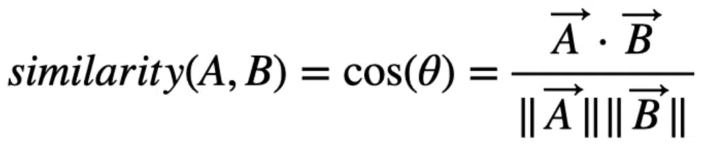
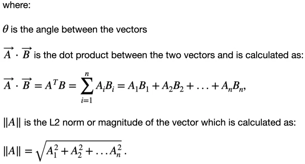
The cosine similarity divides the vector dot product vectors by the Euclidean norm product or vector magnitudes. The similarity can be any value between -1 and +1.

Cosine Distance

The cosine distance is a complement to the cosine similarity in positive space and is defined as:

Visual Description of Cosine Similarity

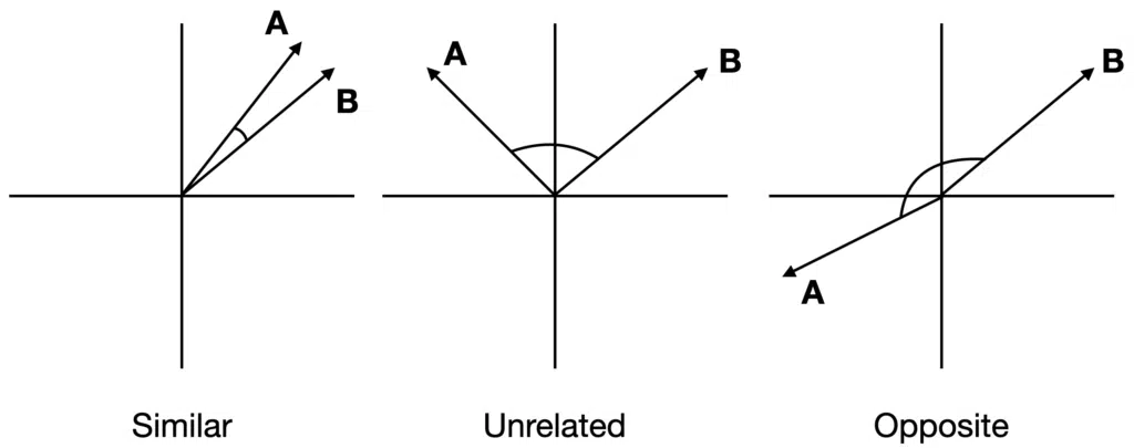
Suppose the angle between two vectors is less than 90 degrees and closer to zero; the cosine similarity measurement will be close to 1. Therefore A and B are more similar to each other. If the angle between the two vectors is 90 degrees, the cosine similarity will have a value of 0; this means that the two vectors are orthogonal and have no correlation between them. The cos($latex \theta$) value can be in the range [-1, 1]. If the angle is much greater than 90 degrees and close to 180 degrees, the similarity value will be close to -1, indicating strongly opposite vectors or no similarity between them.

Numerical Example of Cosine Similarity

To illustrate how we can use cosine similarity, let’s look at an example of document similarity. Thousands of attributes can represent a document, each recording the frequency of a particular word (such as a keyword) or phrase in the document. Therefore, we can represent each document by a term-frequency vector. In the table below, we show two examples of documents containing keywords from the Star Wars franchise.

Document ID	Jedi	Falcon	Force	Droid	Padawan	Nerfherder	Sith	Podracing	Lightsaber
doc_1	5	0	3	0	2	0	0	2	0
doc_2	3	0	2	0	1	1	0	1	0

Term-frequency vectors are typically very long and consist of many zero values. Any two term-frequency vectors may have many 0 values in common, meaning that the corresponding documents do not have many words in common, but this does not mean the two documents are similar. Cosine similarity is beneficial for document similarity because it ignores zero-matches and focuses on the words that the two documents have in common.

Suppose that x and y are the two term-frequency vectors for doc_1 and doc_2; we can calculate the cosine similarity as follows:

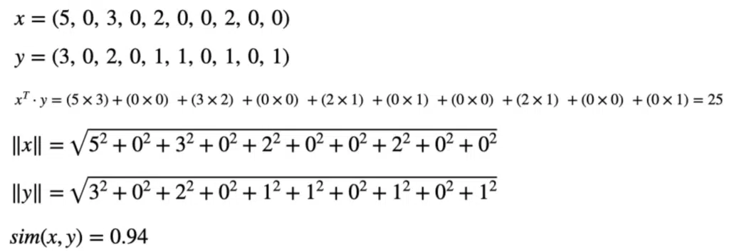
Using the cosine similarity, we can consider the two documents to be very similar.

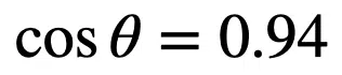
The angle between the vectors can be calculated as:

Python Example of Cosine Similarity

We can use several of the many popular Python libraries for data science and machine learning tasks to demonstrate cosine similarity. In this example, we will use NumPy and scikit-learn. Consider three text documents, we want to compute the cosine similarity between them:

doc_1 = "machine learning is a subset of artificial intelligence"

doc_2 = "machine learning will change the world"

doc_3 = "machine learning engineers build self-running artificial intelligence systems"

corpus = [doc_1, doc_2, doc_3]

We use scikit-learn to vectorized the documents. We can use Pandas to obtain a DataFrame containing the frequencies of the terms in each document.

from sklearn.feature_extraction.text import CountVectorizer

import pandas as pd

count_vectorizer = CountVectorizer(stop_words='english')

count_vectorizer = CountVectorizer()

sparse_matrix = count_vectorizer.fit_transform(corpus)

doc_term_matrix = sparse_matrix.todense()

df = pd.DataFrame(doc_term_matrix, columns=count_vectorizer.get_feature_names(), index=['doc_1', 'doc_2', 'doc_3'])

print(df)

        artificial  build  change  engineers ...  systems  the  will  world
doc_1           1      0       0          0  ...        0    0     0      0
doc_2           0      0       1          0  ...        0    1     1      1
doc_3           1      1       0          1  ...        1    0     0      0

[3 rows x 16 columns]

We can define a function that takes two vectors and returns the cosine similarity. The comments in the function detail the steps that match up to the numeric example above.

def cosine_similarity(a, b):

    # Ensure length of the two vectors a and b are the same

    if len(a) != len(b):

        return None

     # Compute the dot product between a and b

     import numpy as np

     dot_product = np.dot(a, b)

     # Compute the L2 norms (magnitudes) of a and b

     l2_norm_a = np.sqrt(np.sum(a**2))

     l2_norm_b = np.sqrt(np.sum(b**2))

     #Compute the cosine similarity

     cosine_similarity = dot_product / (l2_norm_a * l2_norm_b)

     return cosine_similarity

We need to convert the vectors from matrices to arrays to feed them to our cosine similarity function. Then, we can compute the cosine similarity between the vectors.

X = sparse_matrix.toarray()

sim_1_2 = cosine_similarity(X[0, :], X[1, :])

sim_1_3 = cosine_similarity(X[0, :], X[2, :])

sim_2_3 = cosine_similarity(X[1, :], X[2, :])

print('cosine similarity between doc_1 and doc_2: ', sim_1_2)

print('cosine similarity between doc_1 and doc_3: ', sim_1_3)

print('cosine similarity between doc_2 and doc_3: ', sim_2_3)

cosine similarity between doc_1 and doc_3:  0.3086066999241838

cosine similarity between doc_1 and doc_3:  0.5039526306789696

cosine similarity between doc_2 and doc_3:  0.2721655269759087

If we do not want to write our code, we can use cosine similarity functions defined in popular Python libraries. These include the scikit-learn cosine_similarity function as shown below:

from sklearn.metrics.pairwise import cosine_similarity as cos_sim
cos_sim_1_2 = cos_sim([X[0,:], X[1,:]])
print('cosine similarity between doc_1 and doc_2 is: \n', cos_sim_1_2)

cosine similarity between doc_1 and doc_2 is: 
 [[1.        0.3086067]
 [0.3086067 1.       ]]

Differences Between Cosine and Jaccard Similarity

We define Jaccard similarity as the intersection divided by the size of the union of two sets. Cosine Similarity calculates similarity by measuring the cosine of the angle between two vectors. Jaccard similarity takes only the unique set of words for each document, while cosine similarity takes the total length of term frequency vectors. If the frequency of one or more words changes, the cosine similarity changes, but the Jaccard similarity does not. Jaccard similarity is suitable for cases where duplication is not essential; cosine similarity is ideal for cases where the frequency of terms is critical when analyzing text similarity.

Soft Cosine Similarity

A soft cosine or soft similarity between two vectors considers similarities between pairs of features. Think of soft cosine similarity as a generalization of the cosine similarity that can account for semantic similarity. This method allows us to assess the similarity between two documents in a meaningful way, even when they have no words in common. It uses a measure of similarity between words derived from vector embeddings of words, for example, Word2Vec. The intuition behind the method is that we compute the standard cosine similarity assuming the document vectors are in a non-orthogonal basis. We derive the angle between two basis vectors from the angle between the word2vec embeddings of the corresponding corresponding corresponding words. Below is a graphic of the mapping of semantically similar sentences.

Python Example of Soft Cosine Measure

To use Soft Cosine Measure (SCM) in Python, you will need to use word embeddings. You can train your Word2Vec model, but for this example, we will use an existing Word2Vec model provided by Gensim. There are several Python libraries we need before starting:

• logging – for printing out Gensim logs to console
• nltk – for English stopwords
• gensim – for Bag-of-words method, TF-IDF (term frequency-inerse document frequency) model, and Word2Vec model

We start by importing logging and defining our three sentences, which serve as our documents. The first two sentences have similar content related to machine learning. Therefore the SCM should be high. By contrast, the third sentence is not related to the first two; the SCM should be lower.

import logging

logging.basicConfig(format='%(asctime)s : %(levelname)s : %(message)s', level=logging.INFO)

doc_1 = "machine learning is a subset of artificial intelligence"

doc_2 = "machine learning will change the world"

doc_3 = "I find your lack of faith disturbing"

Once we have the documents defined, we can preprocess them by removing stopwords (“the”, “to” “and”, etc.), as these do not contribute information in the sentences.

from nltk.corpus import stopwords

from nltk import download

download('stopwords')

stop_words = stopwords.words('english')

def pre_process(sentence):
    return[word for word in sentence.lower().split() if word not in stop_words]

doc_1 = pre_process(doc_1)

doc_2 = pre_process(doc_2)

doc_3 = pre_process(doc_3)


Now we build a dictionary and a TF-IDF model, which requires the documents in the bag-of-words format. Think of Bag-of-words as a frequency count for the words in a sentence or document.

from gensim.corpora import Dictionary

docs = [doc_1, doc_2, doc_3]

dictionary = Dictionary(docs)

doc_1 = dictionary.doc2bow(doc_1)

doc_2 = dictionary.doc2bow(doc_2)

doc_3 = dictionary.doc2bow(doc_3)

from gensim.models import TfidfModel

docs = [doc_1, doc_2, doc_3]

tfidf = TfidfModel[docs]

doc_1 = tfidf[doc_1]

doc_2 = tfidf[doc_2]

doc_3 = tfidf[doc_3]


TF-IDF is a statistical measure that evaluates how relevant a word is to a document in a collection of documents. We calculate the measure by multiplying two metrics: how many times a word appears in a document and the inverse document frequency across a set of documents. TF-IDF is useful for automated text analysis and scoring words in machine learning algorithms for Natural Language Processing.

As mentioned earlier, we need to use pre-trained word embeddings. We can download the embedding using Gensim’s downloader API and load the embeddings into a Gensim Word2Vec model class. We build a term similarity matrix using the embeddings. Note that this step requires a lot of memory (~ 1GB).

The WordEmbeddingSimilarityIndex model is a term similarity index that computes cosine similarities between word embeddings. The term similarity matrix takes in the dictionary created earlier, the term similarity index and the TF-IDF measure.

import gensim.downloader as api
model = api.load('word2vec-google-news-300')

from gensim.similarities import SparseTermSimilarityMatrix, WordEmbeddingSimilarityIndex
termsim_index = WordEmbeddingSimilarityIndex(model)
termsim_matrix = SparseTermSimilarityMatrix(termsim_index, dictionary, tfidf)

We can now compute the SCM using the inner product on the TF-IDF vectors for documents 1 and 2

similarity = termsim_matrix.inner_product(doc_1, doc_2 normalized=(True, True))
print('similarity = %.4f' % similarity)


similarity = 0.0999

If we try to compute the SCM for two completely unrelated sentences, we get a much smaller value:

similarity = termsim_matrix.inner_product(doc_1, doc_3 normalized=(True, True))
print('similarity = %.4f' % similarity)

similarity = 0.0000

Summary

Congratulations! You now understand the mathematics behind cosine similarity and why it is helpful for similarity measurement tasks. Soft cosine similarity is a great feature for document classification and clustering using word vectors. You can calculate the cosine similarity of two vectors by hand, write a Python function, or import a scientific computing library.

If you want to learn more about calculating the distance between vectors or points on a plane, visit the article on Manhattan Distance.

To calculate the cosine similarity in R, go to the article: How to Calculate Cosine Similarity in R

If you want to learn more about natural language processing, you can go to the paper readings for BERT, XLNet, and GPT-3.

Have fun and happy researching!